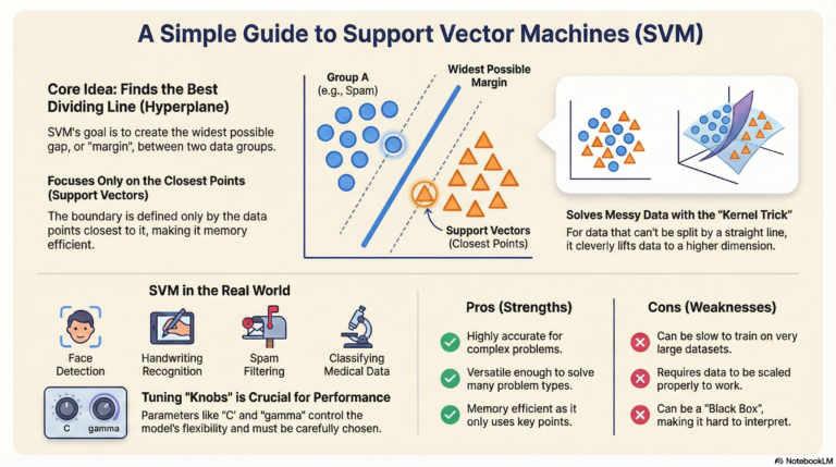
Support Vector Machine (SVM) is a supervised machine learning algorithm used mostly for classification.

Imagine you have a table with Red Apples and Green Oranges mixed together. You want to put a stick (a line) on the table to separate them perfectly.

SVM finds the best stick (line) to separate the two groups.

• It doesn’t just pick any line; it picks the line that has the widest gap (margin) between the fruits.
• This wide gap makes the model stronger and better at guessing new, unseen fruits.

🗝️ Key Concepts (Simple Words)

1. Hyperplane (The Decision Boundary):
   • This is the line that separates the data.
   • If you are drawing on paper (2D), it is a Line.
   • If you are in 3D (like a cube), it is a flat Plane.
   • We just call it a “Hyperplane” to cover all dimensions.
2. Support Vectors:
   • These are the “brave” data points.
   • They are the specific apples and oranges that are closest to the separating line.
   • SVM only cares about these points! If you move the other fruits far away, the line doesn’t change. But if you move a Support Vector, the line moves.
3. Margin:
   • This is the “safe zone” or the street between the two groups.
   • SVM tries to make this street as wide as possible.
   • A wider street means the groups are clearly separate.

🌀 Linear vs. Non-Linear SVM (The Kernel Trick)

Sometimes, you cannot separate the data with a straight line. Imagine the apples are in the middle and the oranges are in a circle around them. A straight line won’t work.

• Linear SVM: Used when data can be split with a straight line.
• Non-Linear SVM: Used when the data is messy and needs a curved line.

🔹 The Kernel Trick: Instead of trying to draw a curved line on paper, the Kernel Trick “lifts” the data into a higher dimension (like lifting the oranges up into the air) so that we can slide a flat sheet between them.

• RBF (Radial Basis Function): The most popular kernel. It creates smooth, curved boundaries. It is the default “magic spell” for complex data.

⚙️ Tuning the Knobs (Hyperparameters)

In the code, we use parameters to control how the model behaves.

1. C (Regularization Parameter):

• Question: Do we want to be strict or flexible?
• High C (Strict): We want to classify every training point correctly. The margin will be narrow. Risk: Overfitting (too sensitive to noise).
• Low C (Flexible): We allow some mistakes to get a bigger, wider margin. Risk: Underfitting.

2. Gamma:

• Question: How far does the influence of a single data point reach?
• High Gamma: Points reach only a very short distance. The boundary is very wiggly and tight around specific points.
• Low Gamma: Points reach far away. The boundary is smoother and more general.

Support Vector Machines (SVM)

💻 Python Code Breakdown

🩺 Breast Cancer Classification using SVM

This program uses Support Vector Machine (SVM) to classify breast cancer tumors as Malignant (Cancer) or Benign (Non-cancer).

📦 Step 0: Import Required Libraries

from sklearn.datasets import load_breast_cancer
from sklearn.svm import SVC
from sklearn.preprocessing import StandardScaler
from sklearn.pipeline import Pipeline
from sklearn.metrics import accuracy_score, classification_report
from sklearn.model_selection import train_test_split

📌 Note:
train_test_split is correctly imported here (you already pointed out it was missing earlier — good observation).

📊 Step 1: Load the Dataset

data = load_breast_cancer()
X = data.data      # Input features (tumor measurements)
y = data.target    # Target labels (0 = malignant, 1 = benign)

• Dataset contains real medical measurements
• Goal: Predict whether a tumor is cancerous or not

✂️ Step 2: Split the Data

X_train, X_test, y_train, y_test = train_test_split(
    X, y, test_size=0.2, random_state=42, stratify=y
)

• 80% training, 20% testing
• stratify=y ensures:
  • Same malignant/benign ratio in both train and test sets
    ✅ Very important in medical datasets

🔧 Step 3: Create a Pipeline (Very Important!)

model = Pipeline([
    ('scaler', StandardScaler()),
    ('svm', SVC(kernel='rbf', C=1.0, gamma='scale'))
])

Why Pipeline?

SVM works on distance calculations.

• One feature may be 1000
• Another may be 0.01
  ❌ This breaks SVM logic

Pipeline Steps:

1. StandardScaler
   • Scales features to same range (mean=0, std=1)
2. SVC (Support Vector Classifier)
   • kernel='rbf' → handles non-linear data
   • C=1.0 → balance between margin and errors
   • gamma='scale' → safe default for RBF kernel

🏋️ Step 4: Train the Model

model.fit(X_train, y_train)

The SVM learns patterns from the training data.

🔮 Step 5: Make Predictions

y_pred = model.predict(X_test)

The model predicts whether each test sample is malignant or benign.

📈 Step 6: Evaluate the Model

print(f"Accuracy: {accuracy_score(y_test, y_pred):.4f}")
print("\nClassification Report:")
print(classification_report(y_test, y_pred, target_names=data.target_names))

🖥️ Sample Output

Accuracy: 0.9737

Classification Report:
              precision    recall  f1-score   support

   malignant       0.98      0.95      0.96        43
      benign       0.97      0.99      0.98        71

    accuracy                           0.97       114
   macro avg       0.97      0.97      0.97       114
weighted avg       0.97      0.97      0.97       114

🧐 How to Read the Output

🔹 Accuracy = 0.9737

• Model is correct 97.4% of the time
• Very strong performance for medical data

🔴 Malignant (Cancer Cases)

• Recall = 0.95
  • Out of all real cancer patients, 95% were correctly detected
  • ❗ Very important → missing cancer is dangerous (Type II error)

🟢 Benign (Healthy Cases)

• Precision = 0.97
  • When the model says “Benign”, it is correct 97% of the time
  • Fewer false cancer alarms

🚨 Medical ML Insight (Very Important)

In healthcare, high recall for malignant cases is more important than accuracy.
Missing a cancer case is far worse than a false alarm.

🔍 Finding the Best Parameters using Grid Search (SVM)

Support Vector Machines are very sensitive to hyperparameters like C, kernel, and gamma.
So instead of guessing, we use GridSearchCV to systematically try many combinations and choose the best one.

🧠 Code Logic (Simple Explanation)

1️⃣ Define the options to try

We give Grid Search a grid (menu) of values:

• C → Controls strictness of the margin
• kernel → How SVM separates data
• gamma → Controls influence of each data point (for rbf)

2️⃣ GridSearchCV behavior

• Trains every possible combination
• Uses 5-fold cross-validation (cv=5)
• Evaluates performance using accuracy
• Automatically selects the best-performing model

💻 Python Code

from sklearn.model_selection import GridSearchCV

# Define the grid of hyperparameters
param_grid = {
    'svm__C': [0.1, 1, 10],
    'svm__kernel': ['rbf', 'linear'],
    'svm__gamma': ['scale', 'auto']
}

# Run Grid Search
grid_search = GridSearchCV(
    model,
    param_grid,
    cv=5,
    scoring='accuracy'
)

grid_search.fit(X_train, y_train)

# Print best parameters
print("Best Parameters found:", grid_search.best_params_)

⚠️ IMPORTANT NOTE (Very Exam-Relevant)

Because we used a Pipeline:

Pipeline([
    ('scaler', StandardScaler()),
    ('svm', SVC())
])

👉 Parameters must be written as:

stepname__parameter

So:

• svm__C
• svm__kernel
• svm__gamma

❌ C alone will NOT work
✅ svm__C is correct

🖥️ Sample Output

Best Parameters found:
{'svm__C': 10, 'svm__gamma': 'scale', 'svm__kernel': 'rbf'}

🧐 How to Read This Output

• C = 10
  • Strong penalty for misclassification
  • Model fits data more tightly
• Kernel = rbf
  • Handles non-linear decision boundaries well
• Gamma = scale
  • Balanced influence of training points (safe default)

✅ This combination performed best across all 5 folds

✅ Pros and Cons Summary

Pros (Good things)	Cons (Bad things)
Accurate: Works very well for complex classification.	Slow: Takes a long time to train if you have huge amounts of data (like 100,000+ rows).
Memory Efficient: Only remembers the “Support Vectors” (the important points).	Sensitive to Noise: If your data has many errors/outliers, it can confuse the boundary line.
Versatile: The “Kernel Trick” allows it to solve many different shapes of problems.	Hard to Interpret: Unlike a simple decision tree, you can’t easily look inside to see why it made a decision (Black Box).
Scaling: Works great when you have many features (columns).	Needs Scaling: You must scale your data (normalizing numbers), or it will fail badly.

🚀 Real-Life Use Cases

1. Face Detection: Classifying parts of an image as “Face” vs “Not Face”.
2. Email Spam Filtering: “Spam” vs “Inbox”.
3. Handwriting Recognition: Reading numbers written on checks (like zip codes).
4. Bioinformatics: Classifying proteins or predicting cancer types based on gene data.

https://aryugyan.com/auto-draft

About the Author

Aryugyan

Administrator

Visit Website View All Posts