✅ 1. List vs. Tuple — Simple Explanation
List
- A list is like a shopping list.
- You can add, remove, or change items anytime.
- Mutable (changeable).
Tuple
- A tuple is like GPS coordinates (latitude, longitude).
- Once created, you cannot modify it.
- Immutable (not changeable).
- Slightly faster and memory efficient than a list.
When to Use?
- Use List → when data needs modification.
- Use Tuple → when data should stay constant and safe from changes.
✅ Code Example
# A list of daily tasks - we might want to add or remove tasks
daily_tasks = ["email", "meeting", "coding"]
print(f"Original list: {daily_tasks}")

# We can easily change an item
daily_tasks[1] = "code review"
print(f"Modified list: {daily_tasks}")

# A tuple of server coordinates - this should not change
server_location = (40.7128, -74.0060)  # (Latitude, Longitude)
print(f"\nOriginal tuple: {server_location}")

# Trying to change a tuple will cause an error
try:
    server_location[0] = 34.0522
except TypeError as e:
    print(f"Error trying to modify tuple: {e}")
✅ Output
Original list: ['email', 'meeting', 'coding']
Modified list: ['email', 'code review', 'coding']

Original tuple: (40.7128, -74.0060)
Error trying to modify tuple: 'tuple' object does not support item assignment
✅ 2. Dictionary Operations — Simple Explanation
A dictionary stores data as key–value pairs.
You can loop through these pairs and apply conditions to filter the data.
Example:
Looping through user profiles and checking which users are older than 30.
✅ Code Example
# A dictionary where keys are user IDs and values are their profiles
user_profiles = {
    "u101": {"name": "Alice", "age": 34},
    "u102": {"name": "Bob", "age": 25},
    "u103": {"name": "Charlie", "age": 42},
    "u104": {"name": "Diana", "age": 29}
}

# Find all users older than 30
users_over_30 = [
    user_id for user_id, profile in user_profiles.items() if profile["age"] > 30
]

print(f"Users older than 30: {users_over_30}")
✅ Output
Users older than 30: ['u101', 'u103']✅ 3. List Comprehension — Simple Explanation
A list comprehension is a short, readable way to create a list.
It replaces long for loops and makes code cleaner.
Code Example
# The original for loop
squares_loop = []
for x in range(10):
    squares_loop.append(x * x)

# The equivalent list comprehension
squares_comp = [x * x for x in range(10)]

print(f"Using a for loop: {squares_loop}")
print(f"Using a list comprehension: {squares_comp}")
Output
Using a for loop: [0, 1, 4, 9, 16, 25, 36, 49, 64, 81]
Using a list comprehension: [0, 1, 4, 9, 16, 25, 36, 49, 64, 81]
✅ 4. Lambda Functions — Simple Explanation
A lambda function is a small, one-line anonymous function.
It is useful for short operations, especially with filter(), map(), sorted(), reduce(), etc.
Code Example
numbers = [10, -5, 22, -1, 0, 15, -8]

# Use filter() with a lambda function to keep only non-negative numbers
positive_numbers = list(filter(lambda x: x >= 0, numbers))

print(f"Original list: {numbers}")
print(f"List with negatives removed: {positive_numbers}")
Output
Original list: [10, -5, 22, -1, 0, 15, -8]
List with negatives removed: [10, 22, 0, 15]
✅ 5. Set Operations — Simple Explanation
A set is a collection of unique items.
You can do mathematical operations like difference, union, intersection, etc.
Example:
Find customers who are in list A but not in list B.
Code Example
list_a = [101, 102, 103, 104, 105]
list_b = [104, 105, 106, 107]

# Convert lists to sets to perform set operations
set_a = set(list_a)
set_b = set(list_b)

# Find customers in list_a but not in list_b (set difference)
customers_only_in_a = list(set_a - set_b)

print(f"List A: {list_a}")
print(f"List B: {list_b}")
print(f"Customers only in List A: {customers_only_in_a}")
Output
List A: [101, 102, 103, 104, 105]
List B: [104, 105, 106, 107]
Customers only in List A: [101, 102, 103]
✅ 6. Memory Efficiency (Generators)
Simple Explanation:
- A list stores all values in memory at once → uses a lot of memory for large datasets.
- A generator produces values one at a time, only when needed → extremely memory-efficient.
Code Example
import sys

# Create a list of the first 1,000,000 numbers
my_list = [i for i in range(1_000_000)]
print(f"Size of list: {sys.getsizeof(my_list)} bytes")

# Create a generator for the first 1,000,000 numbers
my_generator = (i for i in range(1_000_000))
print(f"Size of generator: {sys.getsizeof(my_generator)} bytes")

# Getting values from a generator
print("\nFirst 5 values from generator:")
for i in range(5):
    print(next(my_generator))
Output
Size of list: 8000056 bytes
Size of generator: 200 bytes

First 5 values from generator:
0
1
2
3
4
✅ 7. Functions
Simple Explanation:
A function is a reusable block of code that:
- takes inputs (arguments)
- performs a task
- returns an output
Code Example
import statistics

def calculate_stats(numbers):
    """Calculates mean, median, and standard deviation for a list of numbers."""
    if not numbers:
        return "The list is empty."

    mean = statistics.mean(numbers)
    median = statistics.median(numbers)
    stdev = statistics.stdev(numbers)

    return {"mean": mean, "median": median, "stdev": stdev}

# Example usage
data = [15, 22, 28, 30, 35, 41, 50]
stats = calculate_stats(data)
print(f"Stats for {data}:")
print(stats)
Output
Stats for [15, 22, 28, 30, 35, 41, 50]:
{'mean': 31.57142857142857, 'median': 30, 'stdev': 11.799713686842571}
✅ *8. args and **kwargs
Simple Explanation:
- *args → collects positional arguments into a tuple
Example:func(1, 2, 3) - **kwargs → collects keyword arguments into a dictionary
Example:func(name="Alice", age=30)
They help create flexible functions.
Code Example
import pandas as pd

def create_dataframe(*args, **kwargs):
    """
    Creates a DataFrame.
    *args = positional arguments
    **kwargs = column data
    """
    print("--- Arguments received ---")
    print(f"Positional args (*args): {args}")
    print(f"Keyword args (**kwargs): {kwargs}")
    print("--------------------------")

    return pd.DataFrame(data=kwargs)

# Example usage
df = create_dataframe(
    "name", "age", "city",  # Positional (*args)
    name=["Alice", "Bob"],  # Keyword (**kwargs)
    age=[34, 25],
    city=["New York", "Los Angeles"]
)

print("Resulting DataFrame:")
print(df)
Output
--- Arguments received ---
Positional args (*args): ('name', 'age', 'city')
Keyword args (**kwargs): {'name': ['Alice', 'Bob'], 'age': [34, 25], 'city': ['New York', 'Los Angeles']}
--------------------------
Resulting DataFrame:
    name  age         city
0  Alice   34     New York
1    Bob   25  Los Angeles
✅ 9. Error Handling
Simple Explanation:
A try...except block lets you run risky code safely.
If an error occurs, Python executes the except block instead of crashing.
Code Example
import pandas as pd

file_path = "data/my_non_existent_file.csv"

try:
    df = pd.read_csv(file_path)
    print("File loaded successfully!")
    print(df.head())

except FileNotFoundError:
    print(f"Error: The file at '{file_path}' was not found.")
    print("Please check the file path and try again.")
Output
Error: The file at 'data/my_non_existent_file.csv' was not found.
Please check the file path and try again.
100 Python practical interview questions
✅ 10. Classes (OOP)
Simple Explanation:
A class is a blueprint for creating objects.
Objects have:
- attributes (data)
- methods (functions)
A DataPipeline class can group extract → transform → load steps.
Code Example
class DataPipeline:
    def __init__(self, source_file):
        """Initializes the pipeline with a source file."""
        self.source_file = source_file
        self.data = None
        print(f"Pipeline initialized for source: {self.source_file}")

    def extract(self):
        print("Step 1: Extracting data...")
        self.data = {"col1": [1, 2], "col2": [3, 4]}
        print("Extraction complete.")

    def transform(self):
        print("Step 2: Transforming data...")
        if self.data:
            self.data["col1"] = [x * 10 for x in self.data["col1"]]
        print("Transformation complete.")

    def load(self):
        print("Step 3: Loading data...")
        if self.data:
            print(f"Data to be loaded: {self.data}")
        print("Load complete.")

# Using the class
print("--- Creating a pipeline instance ---")
pipeline = DataPipeline("sales_data.csv")

print("\n--- Running the pipeline ---")
pipeline.extract()
pipeline.transform()
pipeline.load()
Output
--- Creating a pipeline instance ---
Pipeline initialized for source: sales_data.csv

--- Running the pipeline ---
Step 1: Extracting data...
Extraction complete.
Step 2: Transforming data...
Transformation complete.
Step 3: Loading data...
Data to be loaded: {'col1': [10, 20], 'col2': [3, 4]}
Load complete.
✅ 11. Shallow vs Deep Copy
Simple Explanation
- A shallow copy creates a new object but does NOT copy nested objects.
→ Both the original and the copy share the same nested elements. - A deep copy creates a new object and recursively copies everything inside.
→ The original and copy are completely independent.
Why important for Pandas?
df.copy(deep=False)→ shallow copy, risky.
Changes may reflect in the original DataFrame.df.copy()ordf.copy(deep=True)→ safe, original DataFrame remains untouched.
Code Example
import copy
import pandas as pd

# --- Example with a list of lists ---
original_list = [[1, 2, 3], [4, 5, 6]]

# Shallow copy
shallow_copy_list = copy.copy(original_list)

# Deep copy
deep_copy_list = copy.deepcopy(original_list)

print("--- Modifying a nested list in the SHALLOW copy ---")
shallow_copy_list[0][0] = 99
print(f"Original list: {original_list}")  # Changed!
print(f"Shallow copy: {shallow_copy_list}")

print("\n--- Modifying a nested list in the DEEP copy ---")
deep_copy_list[0][0] = 88
print(f"Original list: {original_list}")  # Unchanged
print(f"Deep copy: {deep_copy_list}")

# --- Example with Pandas DataFrames ---
df_original = pd.DataFrame({'col1': [1, 2], 'col2': [3, 4]})
df_shallow = df_original.copy(deep=False)
df_deep = df_original.copy()

print("\n--- Modifying the SHALLOW DataFrame copy ---")
df_shallow.loc[0, 'col1'] = 99
print(f"Original DataFrame:\n{df_original}")
print(f"Shallow DataFrame:\n{df_shallow}")
Output
--- Modifying a nested list in the SHALLOW copy ---
Original list: [[99, 2, 3], [4, 5, 6]]
Shallow copy: [[99, 2, 3], [4, 5, 6]]

--- Modifying a nested list in the DEEP copy ---
Original list: [[99, 2, 3], [4, 5, 6]]
Deep copy: [[88, 2, 3], [4, 5, 6]]

--- Modifying the SHALLOW DataFrame copy ---
Original DataFrame:
   col1  col2
0     1     3
1     2     4
Shallow DataFrame:
   col1  col2
0    99     3
1     2     4
✅ 12. Working with Files (Reading Large Files)
Simple Explanation
When reading very large files, don’t load the whole file into memory.
Use:
with open(...) as f:
    for line in f:
        ...
This reads one line at a time, which is very memory-efficient.
Code Example
# First, let's create a dummy large file
file_path = "large_file.txt"
with open(file_path, "w") as f:
    for i in range(100):
        f.write(f"This is line number {i+1} of the file.\n")

# Now, read it line by line
print(f"Reading '{file_path}' line by line:")
try:
    with open(file_path, "r") as f:
        for i, line in enumerate(f):
            print(f"Line {i+1}: {line.strip()}")
            if i >= 2:  # Stop after 3 lines
                break

except FileNotFoundError:
    print(f"Error: The file '{file_path}' was not found.")
Output
Reading 'large_file.txt' line by line:
Line 1: This is line number 1 of the file.
Line 2: This is line number 2 of the file.
Line 3: This is line number 3 of the file.
✅ 13. Virtual Environments
Simple Explanation
A virtual environment is an isolated Python environment.
Each project can have its own versions of:
- Python packages
- Dependencies
- Library versions
This prevents version conflicts between projects.
Commands (bash)
# 1. Create a virtual environment named 'my_project_env'
python3 -m venv my_project_env

# 2. Activate the environment
# macOS/Linux:
source my_project_env/bin/activate

# Windows:
# my_project_env\Scripts\activate

# 3. Install packages
(my_project_env) $ pip install pandas numpy

# 4. Deactivate
(my_project_env) $ deactivate
Conceptual Output
$ python --version
Python 3.9.6

$ source my_project_env/bin/activate
(my_project_env) $ python --version
Python 3.9.6

(my_project_env) $ pip list | grep pandas
# No output (not installed)

(my_project_env) $ pip install pandas
Successfully installed pandas-1.5.3

(my_project_env) $ pip list | grep pandas
pandas 1.5.3

(my_project_env) $ deactivate

$ pip list | grep pandas
# No output (global environment)
✅ 14. pathlib Module
Simple Explanation
pathlib provides object-oriented file path handling:
- works on Windows, Linux, macOS
- cleaner and safer than using plain strings
- powerful file operations (
rglob,mkdir,/operator)
Code Example
from pathlib import Path

# Create 'data' directory and sample files
data_dir = Path("data")

data_dir.mkdir(exist_ok=True)
(data_dir / "sales.csv").touch()
(data_dir / "customers.csv").touch()
(data_dir / "reports").mkdir(exist_ok=True)
(data_dir / "reports" / "summary.csv").touch()

# Recursively find all CSV files
print(f"Searching for CSV files in '{data_dir}' and its subdirectories:")
csv_files = list(data_dir.rglob("*.csv"))

for file_path in csv_files:
    print(file_path)
Output
Searching for CSV files in 'data' and its subdirectories:
data/sales.csv
data/customers.csv
data/reports/summary.csv
✅ 15. String Manipulation
Simple Explanation
Pandas provides a .str accessor, which allows applying vectorized string operations to an entire column at once.
For standardizing names:
df['city'].str.title()
Code Example
import pandas as pd

# Create a DataFrame with inconsistent city names
data = {'city': ['new york', 'New York', 'NEW YORK', 'london', 'LONDON', 'Paris']}
df = pd.DataFrame(data)

print("Original DataFrame:")
print(df)

# Standardize using .str.title()
df['city_standardized'] = df['city'].str.title()

print("\nDataFrame after standardization:")
print(df)
Output
Original DataFrame:
         city
0    new york
1    New York
2    NEW YORK
3      london
4      LONDON
5       Paris

DataFrame after standardization:
  city_standardized        city
0          New York    new york
1          New York    New York
2          New York    NEW YORK
3           London      london
4           London      LONDON
5            Paris       Paris
✅ 16. Array Creation (NumPy)
Simple Explanation
np.arange()creates a sequence of numbers (like Pythonrange, but as a NumPy array)..reshape()changes the shape of the array, e.g. from 1D → 2D.
Code
import numpy as np

# np.arange(9) creates a 1D array with numbers 0 to 8
arr_1d = np.arange(9)
print("1D array:")
print(arr_1d)

# Convert to a 3x3 matrix
arr_2d = arr_1d.reshape(3, 3)
print("\nReshaped to 3x3 array:")
print(arr_2d)
Output
1D array:
[0 1 2 3 4 5 6 7 8]

Reshaped to 3x3 array:
[[0 1 2]
 [3 4 5]
 [6 7 8]]
✅ 17. Array Indexing
Simple Explanation
- NumPy uses zero-based indexing.
- Access an element in a 2D array using:
array[row_index, column_index]
Code
import numpy as np

arr = np.array([[10, 20, 30],
                [40, 50, 60],
                [70, 80, 90]])

print("Original array:")
print(arr)

element = arr[1, 2]  # second row, third column → 60
print(f"\nThe element at arr[1, 2] is: {element}")
Output
Original array:
[[10 20 30]
 [40 50 60]
 [70 80 90]]

The element at arr[1, 2] is: 60
✅ 18. Boolean Indexing
Simple Explanation
- Apply a condition to create a
True/Falsemask. - Use the mask to filter only the elements that match the condition.
Code
import numpy as np

arr = np.array([1, 5, 10, 15, 20, 25])
print(f"Original array: {arr}")

mean_val = arr.mean()
print(f"Mean: {mean_val}")

mask = arr > mean_val     # Boolean mask
print(f"Mask: {mask}")

filtered_arr = arr[mask]
print(f"Filtered array: {filtered_arr}")
Output
Original array: [ 1  5 10 15 20 25]
Mean: 12.666666666666666
Mask: [False False False  True  True  True]
Filtered array: [15 20 25]
✅ 19. Vectorization
Simple Explanation
- Vectorization = doing operations on the entire array at once.
- NumPy operations run in fast C code, making them much faster than Python loops.
Code
import numpy as np
import timeit

python_list = list(range(1_000_000))
numpy_array = np.arange(1_000_000)

def python_loop():
    new_list = []
    for x in python_list:
        new_list.append(x * 2)
    return new_list

def numpy_vectorized():
    return numpy_array * 2

time_python = timeit.timeit(python_loop, number=10)
time_numpy = timeit.timeit(numpy_vectorized, number=10)

print(f"Python loop: {time_python:.4f} sec")
print(f"NumPy vectorized: {time_numpy:.4f} sec")
print(f"NumPy is {time_python / time_numpy:.0f}x faster")
Output
Python loop: 0.9753 sec
NumPy vectorized: 0.0061 sec
NumPy is 160x faster
100 Python practical interview questions
✅ 20. Reshaping
Simple Explanation
.reshape()changes the shape of the array.- Total number of elements must match.
- Use
-1to allow NumPy to auto-calculate remaining dimension.
Code
import numpy as np

arr_1d = np.arange(12)
print("Original 1D array:", arr_1d)

arr_3x4 = arr_1d.reshape(3, 4)
print("\nReshaped to 3x4:")
print(arr_3x4)

arr_4x3 = arr_1d.reshape(4, -1)  # NumPy calculates -1 → 3
print("\nReshaped to 4x3 using -1:")
print(arr_4x3)
Output
Original 1D array: [ 0  1  2  3  4  5  6  7  8  9 10 11]

Reshaped to 3x4:
[[ 0  1  2  3]
 [ 4  5  6  7]
 [ 8  9 10 11]]

Reshaped to 4x3 using -1:
[[ 0  1  2]
 [ 3  4  5]
 [ 6  7  8]
 [ 9 10 11]]
✅ 21. Array Operations (Clean & Simple Explanation)
NumPy allows you to perform element-wise mathematical operations on entire arrays without loops.
If two arrays have the same shape, you can:
- Add them using
+ - Multiply them using
* - Subtract them using
- - Divide them using
/
These operations happen element by element.
✔ Code Example
import numpy as np

# Create two 2D arrays of the same shape
arr1 = np.array([[1, 2], [3, 4]])
arr2 = np.array([[5, 6], [7, 8]])

print("Array 1:")
print(arr1)

print("\nArray 2:")
print(arr2)

# Calculate the element-wise sum
sum_arr = arr1 + arr2
print("\nElement-wise sum (arr1 + arr2):")
print(sum_arr)

# Calculate the element-wise product
product_arr = arr1 * arr2
print("\nElement-wise product (arr1 * arr2):")
print(product_arr)
✔ Output
Array 1:
[[1 2]
 [3 4]]

Array 2:
[[5 6]
 [7 8]]

Element-wise sum (arr1 + arr2):
[[ 6  8]
 [10 12]]

Element-wise product (arr1 * arr2):
[[ 5 12]
 [21 32]]
🎯 Why this is useful in data science?
- Fast matrix calculations
- Image processing
- Vectorized ML operations
- Neural network computations
✅ 22. Broadcasting (Simple Explanation)
Broadcasting allows NumPy to perform operations on arrays of different shapes by automatically “stretching” the smaller array so both arrays become compatible.
NumPy does not copy the data — it just treats the smaller array as if it were repeated.
✔ When broadcasting happens
An operation like addition works if:
- Dimensions are equal, or
- One of them is 1, so it can be stretched
✔ Code Example
import numpy as np

# Create a 2D array (3 rows, 1 column)
arr_2d = np.array([[1], [2], [3]])
print("2D Array (3x1):")
print(arr_2d)

# Create a 1D array (1 row, 3 columns)
arr_1d = np.array([10, 20, 30])
print("\n1D Array (1x3):")
print(arr_1d)

# Add them together using broadcasting
result = arr_2d + arr_1d
print("\nResult of broadcasting addition (3x3):")
print(result)
✔ Correct Output
2D Array (3x1):
[[1]
 [2]
 [3]]

1D Array (1x3):
[10 20 30]

Result of broadcasting addition (3x3):
[[11 21 31]
 [12 22 32]
 [13 23 33]]
🎯 Why Broadcasting Is Useful?
- Eliminates loops
- Makes vectorized operations possible
- Important in machine learning (matrix operations)
- Used in image processing, normalization, scaling
✅ 23. Aggregation Functions
Simple Explanation:
NumPy allows you to compute summary statistics like mean, sum, and standard deviation along a specific axis.
- axis = 0 → operate down the columns (output becomes 1 row)
- axis = 1 → operate across the rows (output becomes 1 column)
✔ Code
import numpy as np

# Create a 2D array
arr = np.array([[1, 8, 3],
                [4, 5, 6],
                [7, 2, 9]])
print("Original Array:")
print(arr)

# Calculate the mean for each column (axis=0)
col_mean = np.mean(arr, axis=0)
print(f"\nMean of each column (axis=0): {col_mean}")

# Calculate the sum for each row (axis=1)
row_sum = np.sum(arr, axis=1)
print(f"Sum of each row (axis=1): {row_sum}")

# Calculate the standard deviation for each column (axis=0)
col_std = np.std(arr, axis=0)
print(f"Std deviation of each column (axis=0): {col_std}")
✔ Output
Original Array:
[[1 8 3]
 [4 5 6]
 [7 2 9]]

Mean of each column (axis=0): [4. 5. 6.]
Sum of each row (axis=1): [12 15 18]
Std deviation of each column (axis=0): [2.44948974 2.44948974 2.44948974]
✅ 24. Stacking
Simple Explanation:
Stacking means combining arrays together.
- Vertical stacking (
np.vstack) places arrays on top of each other, increasing the number of rows. - All arrays must have the same number of columns.
✔ Code
import numpy as np

# Create two 2D arrays with the same number of columns
arr1 = np.array([[1, 2, 3],
                 [4, 5, 6]])

arr2 = np.array([[7, 8, 9],
                 [10, 11, 12]])

print("Array 1:")
print(arr1)

print("\nArray 2:")
print(arr2)

# Vertically stack the two arrays
stacked_arr = np.vstack((arr1, arr2))
print("\nVertically stacked array:")
print(stacked_arr)
✔ Output
Array 1:
[[1 2 3]
 [4 5 6]]

Array 2:
[[ 7  8  9]
 [10 11 12]]

Vertically stacked array:
[[ 1  2  3]
 [ 4  5  6]
 [ 7  8  9]
 [10 11 12]]
✅ 25. Linspace vs. Arange
Simple Explanation
np.arange(start, stop, step)
Creates values with a fixed step size.
➝ Stop value is NOT included.np.linspace(start, stop, num)
Creates a fixed number of evenly spaced values.
➝ Stop value IS included.
✔ Use arange when step matters.
✔ Use linspace when number of points matters.
✔ Code
import numpy as np

# Use np.arange to get even numbers from 0 up to (but not including) 10
# The step is 2.
arr_arange = np.arange(0, 10, 2)
print(f"np.arange(0, 10, 2) -> {arr_arange}")

# Use np.linspace to get 5 points evenly spaced between 0 and 10
# The number of points is 5.
arr_linspace = np.linspace(0, 10, 5)
print(f"np.linspace(0, 10, 5) -> {arr_linspace}")
✔ Output
np.arange(0, 10, 2) -> [0 2 4 6 8]
np.linspace(0, 10, 5) -> [ 0.   2.5  5.   7.5 10. ]
26. Creating DataFrames
Simple Explanation
You can build a DataFrame in two main ways:
1. From a dictionary of lists
- Keys → column names
- Lists → column values
- All lists must be the same length
2. From a list of dictionaries
- Each dictionary → one row
- Good for JSON-like data
✔ Code
import pandas as pd

# Method 1: From a dictionary of lists
data_dict = {
    'name': ['Alice', 'Bob', 'Charlie'],
    'age': [25, 30, 35],
    'city': ['New York', 'Los Angeles', 'Chicago']
}
df_from_dict = pd.DataFrame(data_dict)
print("DataFrame from a dictionary of lists:")
print(df_from_dict)

# Method 2: From a list of dictionaries
data_list = [
    {'name': 'David', 'age': 40, 'city': 'Houston'},
    {'name': 'Eve', 'age': 28, 'city': 'Phoenix'},
    {'name': 'Frank', 'age': 45, 'city': 'Philadelphia'}
]
df_from_list = pd.DataFrame(data_list)
print("\nDataFrame from a list of dictionaries:")
print(df_from_list)
✔ Output
DataFrame from a dictionary of lists:
      name  age         city
0    Alice   25     New York
1      Bob   30  Los Angeles
2  Charlie   35      Chicago

DataFrame from a list of dictionaries:
    name  age         city
0  David   40      Houston
1    Eve   28      Phoenix
2  Frank   45  Philadelphia
✅ 27. Reading Data
Simple Explanation
pd.read_csv() is the most common way to load data in Pandas.
You can customize:
- sep=’;’ → if your file uses semicolons instead of commas
- encoding=’latin-1′ → useful for files with special characters like é, ç, ü
- io.StringIO → allows treating a string as a file (good for demos)
Code
import pandas as pd
import io

# Simulate a CSV file with semicolon separator and special characters
csv_data = """id;name;city
1;José;São Paulo
2;François;Paris
3;Jürgen;Berlin
"""

# Use io.StringIO to treat the string as a file
df = pd.read_csv(io.StringIO(csv_data), sep=';', encoding='latin-1')

print("DataFrame read from a semicolon-separated CSV:")
print(df)
Output
DataFrame read from a semicolon-separated CSV:
   id       name         city
0   1       José    São Paulo
1   2  François        Paris
2   3    Jürgen       Berlin
✅ 28. Inspecting Data
Simple Explanation
| Function | What it Does | Why it is Useful |
|---|---|---|
df.head(n) | Shows first n rows | Quick preview of data |
df.info() | Shows columns, non-null counts, datatypes | Detect missing values & datatype issues |
df.describe() | Statistics for numeric columns | Understand distribution & outliers |
Code
import pandas as pd
import numpy as np

# Create a sample DataFrame
data = {'product': ['A', 'B', 'C', 'D', 'E'],
        'sales': [100, 150, np.nan, 200, 50],
        'price': [10.0, 15.0, 12.0, 20.0, 5.0]}

df = pd.DataFrame(data)

print("--- df.head() ---")
print(df.head())

print("\n--- df.info() ---")
df.info()

print("\n--- df.describe() ---")
print(df.describe())
Output
--- df.head() ---
  product  sales  price
0       A  100.0   10.0
1       B  150.0   15.0
2       C    NaN   12.0
3       D  200.0   20.0
4       E   50.0    5.0

--- df.info() ---
<class 'pandas.core.frame.DataFrame'>
RangeIndex: 5 entries, 0 to 4
Data columns (total 3 columns):
 #   Column   Non-Null Count  Dtype
 0   product  5 non-null      object
 1   sales    4 non-null      float64
 2   price    5 non-null      float64
dtypes: float64(2), object(1)
memory usage: 248.0+ bytes

--- df.describe() ---
             sales       price
count    4.000000   5.000000
mean   125.000000  12.400000
std     62.915295   5.176872
min     50.000000   5.000000
25%     87.500000  10.000000
50%    125.000000  12.000000
75%    162.500000  15.000000
max    200.000000  20.000000
✅ 29. Selecting Data
Simple Explanation
df['col']
Selects a single column by name → returns a Series.df.loc[](Label-based)
Uses row/column labels.
The end index IS inclusive.df.iloc[](Integer-based)
Uses row/column positions.
The end index is exclusive.
Code
import pandas as pd

df = pd.DataFrame({'product': ['A', 'B', 'C', 'D'],
                   'sales': [100, 150, 120, 200],
                   'price': [10, 15, 12, 20]},
                  index=['row_one', 'row_two', 'row_three', 'row_four'])

print("Original DataFrame:")
print(df)

# Direct bracket notation to select the 'sales' column
sales_series = df['sales']
print("\nSelecting 'sales' column with df['sales']:")
print(sales_series)

# .loc to select by label (inclusive)
loc_selection = df.loc['row_one':'row_three', 'product':'sales']
print("\nSelecting with df.loc (label-based):")
print(loc_selection)

# .iloc to select by integer position (exclusive)
iloc_selection = df.iloc[0:2, 2]
print("\nSelecting with df.iloc (integer-based):")
print(iloc_selection)
Output
Original DataFrame:
           product  sales  price
row_one          A    100     10
row_two          B    150     15
row_three        C    120     12
row_four         D    200     20

Selecting 'sales' column with df['sales']:
row_one      100
row_two      150
row_three    120
row_four     200
Name: sales, dtype: int64

Selecting with df.loc (label-based):
           product  sales
row_one          A    100
row_two          B    150
row_three        C    120

Selecting with df.iloc (integer-based):
row_one     10
row_two     15
Name: price, dtype: int64
✅ 30. Setting Index
Simple Explanation
- Use
df.set_index('column')to make a column the new index. - Useful when working with:
- time-series data
- faster row lookups with
.loc
inplace=Truemodifies the DataFrame directly.
Code
import pandas as pd

# Create a DataFrame with a 'date' column
df = pd.DataFrame({
    'date': ['2023-01-01', '2023-01-02', '2023-01-03'],
    'sales': [200, 250, 180],
    'product': ['X', 'Y', 'Z']
})

print("Original DataFrame:")
print(df)

# Set the 'date' column as the new index
df.set_index('date', inplace=True)

print("\nDataFrame after setting 'date' as the index:")
print(df)
Output
Original DataFrame:
         date  sales product
0  2023-01-01    200       X
1  2023-01-02    250       Y
2  2023-01-03    180       Z

DataFrame after setting 'date' as the index:
            sales product
date
2023-01-01    200       X
2023-01-02    250       Y
2023-01-03    180       Z
✅ 31. Handling Missing Values
Simple Explanation
- Use
df.isnull()to create a boolean DataFrame where:True→ missing value (NaN)False→ present value
- Then apply
.sum()to count how manyTruevalues each column has. - Since True = 1 and False = 0, the sum gives the number of missing values.
Code
import pandas as pd
import numpy as np

# Create a DataFrame with missing values
data = {'name': ['Alice', 'Bob', 'Charlie', 'David'],
        'age': [25, np.nan, 35, 40],
        'city': ['New York', 'Los Angeles', np.nan, 'Chicago'],
        'sales': [200, 150, 300, np.nan]}
df = pd.DataFrame(data)

print("Original DataFrame:")
print(df)

# Find the number of missing values in each column
missing_values = df.isnull().sum()

print("\nNumber of missing values in each column:")
print(missing_values)
Output
Original DataFrame:
      name   age         city  sales
0    Alice  25.0     New York  200.0
1      Bob   NaN  Los Angeles  150.0
2  Charlie  35.0          NaN  300.0
3    David  40.0      Chicago    NaN

Number of missing values in each column:
name     0
age      1
city     1
sales    1
dtype: int64
✅ 32. Dropping / Filling NaNs
Simple Explanation
df.dropna()- Removes rows (or columns) that contain any missing values.
- Use when missing data is rare and losing a few rows is okay.
df.fillna(value)- Replaces missing values with a specified value.
- Common choices:
- mean for numerical data
- median
- mode for categorical data
- Use when you want to keep all rows and handle missing data logically.
Code
import pandas as pd
import numpy as np

df = pd.DataFrame({'A': [1, 2, np.nan, 4],
                   'B': [5, np.nan, np.nan, 8],
                   'C': [9, 10, 11, 12]})

print("Original DataFrame:")
print(df)

# --- dropna: remove any rows with missing values ---
df_dropped = df.dropna()
print("\nDataFrame after dropna():")
print(df_dropped)

# --- fillna: replace NaN with the mean of each column ---
df_filled = df.fillna(df.mean())
print("\nDataFrame after fillna(df.mean()):")
print(df_filled)
Output
Original DataFrame:
     A    B   C
0  1.0  5.0   9
1  2.0  NaN  10
2  NaN  NaN  11
3  4.0  8.0  12

DataFrame after dropna():
     A    B   C
0  1.0  5.0   9
3  4.0  8.0  12

DataFrame after fillna(df.mean()):
     A    B   C
0  1.0  5.0   9
1  2.0  6.5  10
2  2.5  6.5  11
3  4.0  8.0  12
✅ 33. Conditional Replacement
Simple Explanation
- Use boolean indexing with
.locto efficiently replace values based on a condition. - Steps:
- Create a condition, e.g.,
df['inventory'] < 0→ returns a boolean Series. - Use
.loc[condition, 'column']to select only the rows that satisfy the condition. - Assign the new value to those rows.
- Create a condition, e.g.,
Code
import pandas as pd

df = pd.DataFrame({'product': ['A', 'B', 'C', 'D'],
                   'inventory': [50, -10, 120, -5]})

print("Original DataFrame:")
print(df)

# Replace all negative values in the 'inventory' column with 0
df.loc[df['inventory'] < 0, 'inventory'] = 0

print("\nDataFrame after replacing negative values:")
print(df)
Output
Original DataFrame:
  product  inventory
0       A         50
1       B        -10
2       C        120
3       D         -5

DataFrame after replacing negative values:
  product  inventory
0       A         50
1       B          0
2       C        120
3       D          0
✅ 34. Data Types (Currency to Numeric)
Simple Explanation
To convert a currency string like '$1,200.50' to a numeric type:
- Clean the string: remove
$and,. - Convert to numeric: use
pd.to_numeric()to make it a float.
Code
import pandas as pd

df = pd.DataFrame({'item': ['Laptop', 'Mouse'],
                   'price': ['$1,200.50', '$25.00']})

print("Original DataFrame:")
print(df)
print("\nData types:")
print(df.info())

# 1. Remove '$' and ',' using .str.replace()
df['price_cleaned'] = df['price'].str.replace('$', '').str.replace(',', '')

# 2. Convert cleaned string column to numeric (float)
df['price_numeric'] = pd.to_numeric(df['price_cleaned'])

print("\nDataFrame after conversion:")
print(df[['item', 'price_numeric']])
print("\nNew data types:")
print(df[['item', 'price_numeric']].info())
Output
Original DataFrame:
    item      price
0  Laptop  $1,200.50
1   Mouse     $25.00

Data types:
<class 'pandas.core.frame.DataFrame'>
RangeIndex: 2 entries, 0 to 1
Data columns (total 2 columns):
 #   Column  Non-Null Count  Dtype
---  ------  --------------  -----
 0   item    2 non-null      object
 1   price   2 non-null      object
dtypes: object(2)
memory usage: 160.0+ bytes
None

DataFrame after conversion:
    item  price_numeric
0  Laptop        1200.50
1   Mouse           25.00

New data types:
<class 'pandas.core.frame.DataFrame'>
RangeIndex: 2 entries, 0 to 1
Data columns (total 2 columns):
 #   Column         Non-Null Count  Dtype
---  ------         --------------  -----
 0   item           2 non-null      object
 1   price_numeric  2 non-null      float64
dtypes: float64(1), object(1)
memory usage: 160.0+ bytes
None
✅ 35. Removing Duplicates
Simple Explanation
- Use
df.drop_duplicates()to remove duplicate rows. - Parameters:
subset: Specify which columns to consider when identifying duplicates.keep: Decide which duplicate to keep:'first'→ keeps the first occurrence'last'→ keeps the last occurrenceFalse→ removes all duplicates
- Useful for cleaning data where repeated entries are not needed.
Code
import pandas as pd

df = pd.DataFrame({
    'user_id': [1, 2, 1, 3, 2],
    'product_id': ['A', 'B', 'A', 'C', 'B'],
    'transaction_id': [101, 102, 103, 104, 105]
})

print("Original DataFrame:")
print(df)

# Remove duplicate rows based on 'user_id' and 'product_id'
# Keep the first occurrence of each duplicate
df_unique = df.drop_duplicates(subset=['user_id', 'product_id'], keep='first')

print("\nDataFrame after removing duplicates based on 'user_id' and 'product_id':")
print(df_unique)
Output
Original DataFrame:
   user_id product_id  transaction_id
0        1          A             101
1        2          B             102
2        1          A             103
3        3          C             104
4        2          B             105

DataFrame after removing duplicates based on 'user_id' and 'product_id':
   user_id product_id  transaction_id
0        1          A             101
1        2          B             102
3        3          C             104
✅ 36. Applying Functions
Simple Explanation
df.apply(func, axis=…): Applies a function to columns (axis=0) or rows (axis=1). Useful for operations involving multiple columns/rows.series.map(func): Applies a function element-wise to a single column. Great for simple transformations or mapping values.df.applymap(func): Applies a function element-wise to every element in the entire DataFrame. Useful for universal element-wise transformations.
Code
import pandas as pd

df = pd.DataFrame({'A': [1, 2, 3], 'B': [4, 5, 6]})
print("Original DataFrame:")
print(df)

# --- df.apply() example: Sum of columns for each row ---
df['row_sum'] = df.apply(lambda row: row.A + row.B, axis=1)
print("\nAfter df.apply() to get row sum:")
print(df)

# --- series.map() example: Map numbers to words ---
number_map = {1: 'one', 2: 'two', 3: 'three'}
df['A_word'] = df['A'].map(number_map)
print("\nAfter series.map() to convert numbers to words:")
print(df)

# --- df.applymap() example: Convert all numbers to strings ---
df_str = df.applymap(str)
print("\nAfter df.applymap() to convert all elements to strings:")
print(df_str)
Output
Original DataFrame:
   A  B
0  1  4
1  2  5
2  3  6

After df.apply() to get row sum:
   A  B  row_sum
0  1  4        5
1  2  5        7
2  3  6        9

After series.map() to convert numbers to words:
   A  B  row_sum A_word
0  1  4        5     one
1  2  5        7     two
2  3  6        9   three

After df.applymap() to convert all elements to strings:
   A  B row_sum A_word
0  1  4      5    one
1  2  5      7    two
2  3  6      9  three
36. Applying Functions
Simple Explanation
df.apply(func, axis=…)- Applies a function across rows (
axis=1) or columns (axis=0). - Useful when a calculation involves multiple columns or rows.
- Applies a function across rows (
series.map(func)- Applies a function element-wise to a single column (Pandas Series).
- Good for simple transformations, e.g., mapping values to words or categories.
df.applymap(func)- Applies a function element-wise to every value in the DataFrame.
- Useful for universal transformations, like converting all numbers to strings.
Code Example
import pandas as pd

# Create a simple DataFrame
df = pd.DataFrame({'A': [1, 2, 3], 'B': [4, 5, 6]})
print("Original DataFrame:")
print(df)

# --- 1. df.apply(): Sum of columns for each row (axis=1) ---
df['row_sum'] = df.apply(lambda row: row.A + row.B, axis=1)
print("\nAfter df.apply() to get row sum:")
print(df)

# --- 2. series.map(): Map numbers to words ---
number_map = {1: 'one', 2: 'two', 3: 'three'}
df['A_word'] = df['A'].map(number_map)
print("\nAfter series.map() to convert numbers to words:")
print(df)

# --- 3. df.applymap(): Convert all elements to strings ---
df_str = df.applymap(str)
print("\nAfter df.applymap() to convert all elements to strings:")
print(df_str)
Output
Original DataFrame:
   A  B
0  1  4
1  2  5
2  3  6

After df.apply() to get row sum:
   A  B  row_sum
0  1  4        5
1  2  5        7
2  3  6        9

After series.map() to convert numbers to words:
   A  B  row_sum A_word
0  1  4        5     one
1  2  5        7     two
2  3  6        9   three

After df.applymap() to convert all elements to strings:
   A  B row_sum A_word
0  1  4      5    one
1  2  5      7    two
2  3  6      9  three
37. String Methods
Simple Explanation
- Use
.straccessor on a Pandas Series to apply string operations. - You can perform operations like:
.split(),.replace(),.lower(),.upper(),.contains(), etc.
- Example Use Case: Extracting the domain from an email by splitting the string at the ‘@’ symbol.
Code Example
import pandas as pd

# Create a sample DataFrame
df = pd.DataFrame({
    'name': ['Alice', 'Bob'],
    'email': ['alice@example.com', 'bob@work-mail.org']
})

print("Original DataFrame:")
print(df)

# --- Extract domain from email ---
# Split the email at '@' and take the second part (index 1)
df['domain'] = df['email'].str.split('@').str[1]

print("\nDataFrame after extracting domain:")
print(df)
Output
Original DataFrame:
    name              email
0  Alice    alice@example.com
1    Bob  bob@work-mail.org

DataFrame after extracting domain:
    name              email          domain
0  Alice    alice@example.com      example.com
1    Bob  bob@work-mail.org    work-mail.org
💡 Tip:
The .str accessor is powerful for all kinds of string manipulations in a DataFrame column. You can chain multiple string methods like:
df['domain'].str.upper().str.replace('-', '_')38. GroupBy
Simple Explanation
- GroupBy splits a DataFrame into groups based on some criteria.
- You can apply a function (like
sum,mean,count) to each group independently. - Finally, results are combined into a new data structure (Series or DataFrame).
Steps:
- Split the data into groups (
.groupby()). - Apply an aggregation or transformation (
.sum(),.mean(), etc.). - Combine the results into a new object.
Code Example
import pandas as pd

# Create a sample sales DataFrame
data = {
    'region': ['East', 'West', 'East', 'West', 'East', 'West'],
    'product': ['A', 'B', 'A', 'C', 'B', 'C'],
    'sales': [100, 150, 120, 200, 80, 250]
}
df = pd.DataFrame(data)

print("Original DataFrame:")
print(df)

# --- Group by 'region' and calculate total sales ---
total_sales_by_region = df.groupby('region')['sales'].sum()

print("\nTotal sales for each region:")
print(total_sales_by_region)
Output
Original DataFrame:
  region product  sales
0   East       A    100
1   West       B    150
2   East       A    120
3   West       C    200
4   East       B     80
5   West       C    250

Total sales for each region:
region
East    300
West    600
Name: sales, dtype: int64
💡 Tip:
You can also group by multiple columns and use different aggregation functions:
df.groupby(['region', 'product'])['sales'].mean()39. Aggregations (Most Common Product)
Simple Explanation
- When working with grouped data, you often want to know which item appears most frequently in each group.
- Steps:
- Use
.groupby()to group by a column (e.g.,region). - Use
.apply()with a custom function on the grouped column. - Inside the function:
.value_counts()counts occurrences of each unique value..idxmax()returns the value with the highest count.
- Use
Code Example
import pandas as pd

df = pd.DataFrame({
    'region': ['East', 'West', 'East', 'West', 'East', 'West', 'East'],
    'product': ['A', 'B', 'A', 'C', 'B', 'C', 'A']  # Product 'A' is most common in East
})

print("Original DataFrame:")
print(df)

# Group by 'region' and find the most frequent product in each group
most_common_product = df.groupby('region')['product'].apply(lambda x: x.value_counts().idxmax())

print("\nMost common product in each region:")
print(most_common_product)
Output
Original DataFrame:
  region product
0   East       A
1   West       B
2   East       A
3   West       C
4   East       B
5   West       C
6   East       A

Most common product in each region:
region
East     A
West     C
Name: product, dtype: object
💡 Tip:
- You can also use
.agg()with a lambda for more complex summaries. - For example, to get both most common product and its count:
df.groupby('region')['product'].agg(lambda x: x.value_counts().idxmax())40. Pivot Table
Simple Explanation
- A pivot table reshapes data to summarize it.
- You select:
- Index (rows) → unique values of one column.
- Columns → unique values of another column.
- Values → data to fill in the table.
- You can also specify an aggregation function (
aggfunc) likemean,sum,count.
Code Example
import pandas as pd

data = {'region': ['East', 'West', 'East', 'West', 'East', 'West'],
        'product': ['A', 'B', 'A', 'C', 'B', 'C'],
        'sales': [100, 150, 120, 200, 80, 250]}
df = pd.DataFrame(data)

print("Original DataFrame:")
print(df)

# Create a pivot table
pivot = pd.pivot_table(df,
                       index='region',      # Rows
                       columns='product',   # Columns
                       values='sales',      # Values to fill
                       aggfunc='mean')      # Aggregation function

print("\nPivot table of average sales:")
print(pivot)
Output
Original DataFrame:
  region product  sales
0   East       A    100
1   West       B    150
2   East       A    120
3   West       C    200
4   East       B     80
5   West       C    250

Pivot table of average sales:
product      A      B      C
region
East      110.0   80.0    NaN
West        NaN  150.0  225.0
💡 Tip:
NaNmeans no data exists for that combination (e.g., East has no C sales in this example).
41. Melting Data
Simple Explanation
- Melting converts a DataFrame from wide to long format.
- Multiple columns are combined into two columns:
variable→ original column names.value→ values from those columns.
- Useful for plotting or reshaping data for analysis.
Code Example
import pandas as pd

# Wide format DataFrame
df_wide = pd.DataFrame({
    'student': ['Alice', 'Bob'],
    'math_score': [90, 85],
    'english_score': [95, 80]
})

print("Original WIDE format DataFrame:")
print(df_wide)

# Melt to long format
df_long = pd.melt(df_wide,
                  id_vars=['student'],         # Column to keep
                  value_vars=['math_score', 'english_score'],  # Columns to unpivot
                  var_name='subject',          # Name of new 'variable' column
                  value_name='score')          # Name of new 'value' column

print("\nMelted to LONG format DataFrame:")
print(df_long)
Output
Original WIDE format DataFrame:
  student  math_score  english_score
0   Alice          90             95
1     Bob          85             80

Melted to LONG format DataFrame:
  student         subject  score
0   Alice     math_score     90
1     Bob     math_score     85
2   Alice  english_score     95
3     Bob  english_score     80
💡 Tip:
- Melting is the opposite of a pivot table. After melting, you can easily group, aggregate, or plot the long-format data.
42. Merging DataFrames
Simple Explanation
- Merging combines two DataFrames based on a common key column.
- Common join types:
| Join Type | Description |
|---|---|
| Inner | Keeps only rows where the key exists in both DataFrames. |
| Left | Keeps all rows from the left DataFrame and adds matching rows from the right. Non-matches become NaN. |
| Right | Keeps all rows from the right DataFrame and adds matching rows from the left. Non-matches become NaN. |
| Outer | Keeps all rows from both DataFrames. Non-matches on either side become NaN. |
Code Example
import pandas as pd

# Create two DataFrames
df1 = pd.DataFrame({'id': [1, 2, 3], 'name': ['Alice', 'Bob', 'Charlie']})
df2 = pd.DataFrame({'id': [2, 3, 4], 'city': ['New York', 'Chicago', 'Houston']})

print("DataFrame 1:")
print(df1)
print("\nDataFrame 2:")
print(df2)

# Inner Join
inner_join = pd.merge(df1, df2, on='id', how='inner')
print("\n--- Inner Join ---")
print(inner_join)

# Left Join
left_join = pd.merge(df1, df2, on='id', how='left')
print("\n--- Left Join ---")
print(left_join)

# Outer Join
outer_join = pd.merge(df1, df2, on='id', how='outer')
print("\n--- Outer Join ---")
print(outer_join)
Output
DataFrame 1:
   id     name
0   1    Alice
1   2      Bob
2   3  Charlie

DataFrame 2:
   id      city
0   2  New York
1   3   Chicago
2   4   Houston

--- Inner Join ---
   id     name      city
0   2      Bob  New York
1   3  Charlie   Chicago

--- Left Join ---
   id     name      city
0   1    Alice       NaN
1   2      Bob  New York
2   3  Charlie   Chicago

--- Outer Join ---
   id     name      city
0   1    Alice       NaN
1   2      Bob  New York
2   3  Charlie   Chicago
3   4      NaN   Houston
💡 Tips:
- Always specify the key column (
on='id') for clarity. - Choose the join type depending on whether you want to keep unmatched rows.
Right Joinworks similarly toLeft Joinbut keeps all rows from the right DataFrame.
43. Concatenation
Simple Explanation
Concatenation stacks DataFrames either vertically or horizontally:
| Type | Description |
|---|---|
| Vertical (axis=0) | Stacks DataFrames on top of each other. Columns must match. Indexes may repeat. |
| Horizontal (axis=1) | Stacks DataFrames side by side. Indexes must match. Columns can be different. |
Code Example
import pandas as pd

# DataFrames for vertical stacking
df1 = pd.DataFrame({'A': ['A0', 'A1'], 'B': ['B0', 'B1']})
df2 = pd.DataFrame({'A': ['A2', 'A3'], 'B': ['B2', 'B3']})

# DataFrame for horizontal stacking
df3 = pd.DataFrame({'C': ['C0', 'C1'], 'D': ['D0', 'D1']}, index=[0, 1])

print("DataFrame 1:")
print(df1)
print("\nDataFrame 2:")
print(df2)

# --- Vertical Stacking ---
vertical_stack = pd.concat([df1, df2])
print("\n--- Vertically Stacked ---")
print(vertical_stack)

# --- Horizontal Stacking ---
horizontal_stack = pd.concat([df1, df3], axis=1)
print("\n--- Horizontally Stacked ---")
print(horizontal_stack)
Output
DataFrame 1:
    A   B
0  A0  B0
1  A1  B1

DataFrame 2:
    A   B
0  A2  B2
1  A3  B3

--- Vertically Stacked ---
    A   B
0  A0  B0
1  A1  B1
0  A2  B2
1  A3  B3

--- Horizontally Stacked ---
    A   B   C   D
0  A0  B0  C0  D0
1  A1  B1  C1  D1
💡 Tips:
- For vertical stacking, mismatched columns will create
NaNfor missing columns. - For horizontal stacking, mismatched indexes will create
NaNfor missing rows. pd.concatis very flexible; you can also useignore_index=Trueto reindex vertically stacked DataFrames.
44. Cross Tabulation
Simple Explanation
pd.crosstab() creates a frequency table that counts how often combinations of two (or more) categorical variables occur. It’s very useful for understanding relationships between categories.
Code Example
import pandas as pd

df = pd.DataFrame({
    'Gender': ['Male', 'Female', 'Female', 'Male', 'Male', 'Female'],
    'Preference': ['A', 'B', 'A', 'A', 'B', 'B']
})

print("Original DataFrame:")
print(df)

# Create a frequency table of Gender vs. Preference
cross_tab = pd.crosstab(df['Gender'], df['Preference'])

print("\nCross-tabulation (Frequency Table):")
print(cross_tab)
Output
Original DataFrame:
   Gender Preference
0    Male          A
1  Female          B
2  Female          A
3    Male          A
4    Male          B
5  Female          B

Cross-tabulation (Frequency Table):
Preference  A  B
Gender
Female      1  2
Male        2  1
Tips
- You can add
margins=Trueto see row and column totals:
pd.crosstab(df['Gender'], df['Preference'], margins=True)Works with more than 2 variables by passing multiple Series.
You can apply aggregation with the values and aggfunc parameters if counting numeric data instead of just frequency.
45. Datetime Conversion
Simple Explanation
To work effectively with dates in Pandas, you need to convert date strings to datetime objects. This allows for easy comparison, filtering, and time-based operations.
Code Example
import pandas as pd

# Create a DataFrame with a date column as strings
df = pd.DataFrame({
    'date': ['2023-10-27', '2023-10-28', '2023-10-29'],
    'sales': [200, 250, 180]
})

print("Original DataFrame:")
print(df)
print("\nData type of 'date' column:", df['date'].dtype)

# Convert the 'date' column to datetime objects
df['date'] = pd.to_datetime(df['date'])

print("\nDataFrame after conversion:")
print(df)
print("\nNew data type of 'date' column:", df['date'].dtype)
Output
Original DataFrame:
         date  sales
0  2023-10-27    200
1  2023-10-28    250
2  2023-10-29    180

Data type of 'date' column: object

DataFrame after conversion:
        date  sales
0 2023-10-27    200
1 2023-10-28    250
2 2023-10-29    180

New data type of 'date' column: datetime64[ns]
46. Time-based Filtering
Simple Explanation
Once the date column is converted and set as the index, you can filter by year, month, or date range using string-based indexing. This is extremely useful for time series data analysis.
Code Example
import pandas as pd

# Create a DataFrame with a DatetimeIndex
date_rng = pd.date_range(start='2022-01-01', end='2023-10-30', freq='D')
df = pd.DataFrame(date_rng, columns=['date'])
df['data'] = range(len(df))
df.set_index('date', inplace=True)

print("Original DataFrame (head):")
print(df.head())

# Select all data from the year 2022
data_2022 = df['2022']
print("\nData from the year 2022 (head):")
print(data_2022.head())

# Select data from a specific month
data_jan_2022 = df['2022-01']
print("\nData from January 2022 (head):")
print(data_jan_2022.head())
Output
Original DataFrame (head):
            data
date
2022-01-01     0
2022-01-02     1
2022-01-03     2
2022-01-04     3
2022-01-05     4

Data from the year 2022 (head):
            data
date
2022-01-01     0
2022-01-02     1
2022-01-03     2
2022-01-04     3
2022-01-05     4

Data from January 2022 (head):
            data
date
2022-01-01     0
2022-01-02     1
2022-01-03     2
2022-01-04     3
2022-01-05     4
Tips
- After conversion, you can easily extract parts of the date:
df['year'] = df.index.year
df['month'] = df.index.month
df['day'] = df.index.day
- Combine filtering with conditions:
df['2022-03':'2022-06'] # Data from March to June 202247. Resampling
Simple Explanation
Resampling is used to change the frequency of time series data:
- Downsampling: Reduce the frequency (e.g., daily → monthly) by aggregating values (
mean,sum,max, etc.). - Upsampling: Increase the frequency (e.g., monthly → daily) by filling or interpolating missing values.
The .resample() method is used on a DatetimeIndex and requires an aggregation function for downsampling.
Code Example
import pandas as pd
import numpy as np

# Create a DataFrame with daily stock prices
date_rng = pd.date_range(start='2023-01-01', periods=90, freq='D')
df_daily = pd.DataFrame(date_rng, columns=['date'])
df_daily['price'] = np.random.randint(100, 150, size=len(date_rng))
df_daily.set_index('date', inplace=True)

print("Original daily data (head):")
print(df_daily.head())

# Downsample daily data to monthly average price
df_monthly = df_daily['price'].resample('M').mean()

print("\nResampled monthly average price:")
print(df_monthly)
Output Example
Original daily data (head):
            price
date
2023-01-01    106
2023-01-02    129
2023-01-03    108
2023-01-04    112
2023-01-05    119

Resampled monthly average price:
date
2023-01-31    124.03
2023-02-28    126.61
2023-03-31    124.64
Name: price, dtype: float64
Tips
- Common frequency codes for
.resample():'D'→ Daily'W'→ Weekly'M'→ Month-end'Q'→ Quarter-end'Y'→ Year-end
- Example of upsampling with forward fill:
df_monthly_upsampled = df_monthly.resample('D').ffill()
- You can combine
.resample()with any aggregation function:
df_daily['price'].resample('W').max() # Weekly maximum48. Rolling Windows
Simple Explanation
A rolling window performs calculations over a fixed-size “window” of consecutive data points that moves across the time series:
- Each window contains a subset of consecutive rows.
- Common uses: moving averages, rolling sums, min/max, standard deviation, etc.
- Example: a 7-day rolling average calculates the average of the current day plus the previous 6 days, then slides forward one day and repeats.
Code Example
import pandas as pd

# Daily sales data
df = pd.DataFrame({
    'date': pd.date_range(start='2023-01-01', periods=15, freq='D'),
    'sales': [10, 20, 15, 30, 25, 40, 35, 50, 45, 60, 55, 70, 65, 80, 75]
})
df.set_index('date', inplace=True)

print("Original daily sales:")
print(df)

# Calculate a 7-day rolling average
df['7_day_rolling_avg'] = df['sales'].rolling(window=7).mean()

print("\nDataFrame with 7-day rolling average:")
print(df)
Output Example
Original daily sales:
            sales
date
2023-01-01     10
2023-01-02     20
2023-01-03     15
2023-01-04     30
2023-01-05     25
2023-01-06     40
2023-01-07     35
2023-01-08     50
2023-01-09     45
2023-01-10     60
2023-01-11     55
2023-01-12     70
2023-01-13     65
2023-01-14     80
2023-01-15     75

DataFrame with 7-day rolling average:
            sales  7_day_rolling_avg
date
2023-01-01     10                 NaN
2023-01-02     20                 NaN
2023-01-03     15                 NaN
2023-01-04     30                 NaN
2023-01-05     25                 NaN
2023-01-06     40                 NaN
2023-01-07     35               25.0
2023-01-08     50               30.0
2023-01-09     45               35.0
2023-01-10     60               40.0
2023-01-11     55               45.0
2023-01-12     70               50.0
2023-01-13     65               55.0
2023-01-14     80               60.0
2023-01-15     75               65.0
Tips
- Window size determines how many rows are included in the calculation.
- The first few rows will often be NaN because the window isn’t full yet.
- You can compute other functions like:
df['7_day_rolling_sum'] = df['sales'].rolling(window=7).sum()
df['7_day_rolling_std'] = df['sales'].rolling(window=7).std()
- Works well for smoothing noisy time series data.
49. Time Deltas
Simple Explanation
A Time Delta represents the difference between two dates or times. In Pandas:
- Subtracting two datetime columns gives a Timedelta Series.
- You can extract useful information such as:
.dt.days→ total days.dt.seconds→ total seconds.dt.total_seconds()→ total duration in seconds
This is very useful for calculating durations, age, or elapsed time between events.
Code Example
import pandas as pd

# Create a DataFrame with two datetime columns
df = pd.DataFrame({
    'start_date': pd.to_datetime(['2023-01-01', '2023-02-15', '2023-03-20']),
    'end_date': pd.to_datetime(['2023-01-10', '2023-03-01', '2023-04-01'])
})

print("Original DataFrame:")
print(df)

# Calculate time difference
df['time_delta'] = df['end_date'] - df['start_date']

# Extract difference in days
df['days_difference'] = df['time_delta'].dt.days

print("\nDataFrame with time difference in days:")
print(df)
Output Example
Original DataFrame:
  start_date   end_date
0 2023-01-01 2023-01-10
1 2023-02-15 2023-03-01
2 2023-03-20 2023-04-01

DataFrame with time difference in days:
  start_date   end_date time_delta  days_difference
0 2023-01-01 2023-01-10    9 days                9
1 2023-02-15 2023-03-01   14 days               14
2 2023-03-20 2023-04-01   12 days               12
Tips
Timedeltacan also be used for arithmetic with dates, e.g., adding/subtracting days:
df['new_date'] = df['start_date'] + pd.Timedelta(days=7)
- Works with hours, minutes, seconds, e.g.,
pd.Timedelta(hours=5). - Ideal for time-based calculations like calculating SLA, age, or subscription durations.
50. Matplotlib Basics (Line Plot)
Simple Explanation
- Line plots visualize trends over a continuous variable (like time).
- Steps:
- Import
matplotlib.pyplot. - Prepare
xandydata. - Use
plt.plot(x, y). - Add labels, title, and show the plot.
- Import
Code Example
import matplotlib.pyplot as plt

# Sample data
years = [2018, 2019, 2020, 2021, 2022]
sales = [15000, 18000, 16000, 22000, 27000]

# Line plot
plt.plot(years, sales)

# Add title and labels
plt.title("Yearly Sales")
plt.xlabel("Year")
plt.ylabel("Sales ($)")

# Display
plt.show()
Output:
A line chart showing sales trends over years with proper labels.
51. Scatter Plot
Simple Explanation
- Scatter plots visualize the relationship or correlation between two numerical variables.
- Use
plt.scatter(x, y).
Code Example
import matplotlib.pyplot as plt

# Sample data
age = [25, 30, 35, 40, 45, 50, 55, 60]
income = [40000, 55000, 60000, 75000, 90000, 110000, 95000, 120000]

# Scatter plot
plt.scatter(age, income)

# Add title and labels
plt.title("Age vs. Income")
plt.xlabel("Age")
plt.ylabel("Annual Income ($)")

# Display
plt.show()
Output:
A scatter plot showing the relationship between age and income (generally positive correlation).
52. Histogram
Simple Explanation
- Histograms show the distribution of a single numerical variable.
- Use
plt.hist(data, bins=number_of_bins)to control granularity.
Code Example
import matplotlib.pyplot as plt
import numpy as np

# Sample data: ages of 100 customers
customer_age = np.random.randint(18, 70, size=100)

# Histogram
plt.hist(customer_age, bins=10, edgecolor='black')

# Add title and labels
plt.title("Distribution of Customer Age")
plt.xlabel("Age")
plt.ylabel("Number of Customers")

# Display
plt.show()
Output:
Histogram showing how customer ages are distributed across 10 bins.
53. Seaborn vs. Matplotlib
Simple Explanation
- Matplotlib: Foundational plotting library. Very flexible, but can require a lot of code for polished plots.
- Seaborn: Built on top of Matplotlib. Simplifies statistical visualization and improves aesthetics.
Key Advantages of Seaborn
- Better Aesthetics: Beautiful default styles.
- Works with DataFrames: Directly use column names from a DataFrame.
sns.scatterplot(x='col1', y='col2', data=df) - Complex Plots Made Easy: Box plots, violin plots, heatmaps, pair plots, etc., are simpler to create than with Matplotlib alone.
54. Box Plot
Simple Explanation
- Box plots show the distribution of a numerical variable across categories.
- Displays median, quartiles, and outliers.
- Seaborn makes it simple with
sns.boxplot().
Code Example
import seaborn as sns
import matplotlib.pyplot as plt
import pandas as pd

# Sample data
data = {'department': ['HR', 'IT', 'Sales', 'HR', 'IT', 'Sales', 'HR', 'IT', 'Sales'],
        'salary': [60000, 90000, 75000, 65000, 110000, 120000, 62000, 95000, 80000]}
df = pd.DataFrame(data)

# Create the box plot
sns.boxplot(x='department', y='salary', data=df)

# Add title
plt.title("Salary Distribution by Department")

# Display
plt.show()
Output:
Three boxes (one per department) showing median, quartiles, and outliers.
55. Heatmap
Simple Explanation
- A heatmap visualizes values in a matrix using colors.
- Often used for correlation matrices.
- Use
df.corr()to compute correlations, thensns.heatmap()to visualize.
Code Example
import seaborn as sns
import matplotlib.pyplot as plt
import pandas as pd

# Sample data
df = pd.DataFrame({'age': [25, 30, 35, 40],
                   'income': [50000, 60000, 75000, 90000],
                   'score': [85, 88, 92, 95]})

# Compute correlation matrix
correlation_matrix = df.corr()

# Create heatmap
sns.heatmap(correlation_matrix, annot=True, cmap='coolwarm')

# Add title
plt.title("Correlation Matrix Heatmap")

# Display
plt.show()
Output:
A 3×3 heatmap showing correlations, with values annotated in each cell and color-coded.
56. Subplots
Simple Explanation
plt.subplots()lets you create multiple plots in a single figure.- Returns a figure object (
fig) and axes object(s) (ax) for plotting individually. - Use ax[i] to access a specific subplot.
figsizecontrols the overall figure size.plt.tight_layout()prevents overlapping elements.
Code Example
import matplotlib.pyplot as plt

# Sample data
years = [2018, 2019, 2020, 2021, 2022]
sales = [150, 180, 160, 220, 270]
profit = [20, 35, 15, 50, 65]

# Create a figure with 1 row and 2 columns of subplots
fig, ax = plt.subplots(1, 2, figsize=(12, 5))

# Plot on the first subplot
ax[0].plot(years, sales)
ax[0].set_title('Yearly Sales')
ax[0].set_xlabel('Year')
ax[0].set_ylabel('Sales ($)')

# Plot on the second subplot
ax[1].bar(years, profit, color='green')
ax[1].set_title('Yearly Profit')
ax[1].set_xlabel('Year')
ax[1].set_ylabel('Profit ($)')

# Adjust layout and display
plt.tight_layout()
plt.show()
Output:
A single figure with two plots side-by-side:
- Left: line plot for sales
- Right: bar chart for profit
57. Customization
Simple Explanation
- Add titles and axis labels using:
plt.title()→ plot titleplt.xlabel()→ x-axis labelplt.ylabel()→ y-axis label
- You can also change colors, markers, line styles, and fonts for further customization.
Code Example
import matplotlib.pyplot as plt

# Sample data
x = [1, 2, 3, 4]
y = [10, 20, 25, 30]

plt.plot(x, y, marker='o', linestyle='--', color='orange')

# Add title and labels
plt.title("My Simple Plot")
plt.xlabel("X-axis Label")
plt.ylabel("Y-axis Label")

# Display the plot
plt.show()
Output:
A line plot with a title, labeled axes, and custom markers and line style.
58. Saving Plots
Simple Explanation
- After creating a Matplotlib plot, save it to a file using
plt.savefig(). - Call
plt.savefig()beforeplt.show(). - File format is determined by the extension:
.png,.pdf,.svg, etc.
Code Example
import matplotlib.pyplot as plt

x = [1, 2, 3, 4]
y = [10, 20, 25, 30]

plt.plot(x, y)
plt.title("Plot to be Saved")

# Save the figure
plt.savefig("my_plot.png")  # PNG file
# plt.savefig("my_plot.pdf")  # PDF file

plt.show()
Output:
- The plot is displayed.
- A file
my_plot.pngis created in the current directory.
59. Interactive Plots
Simple Explanation
- Interactive plots allow hovering, zooming, panning, and selection, which is great for dashboards or web apps.
- Use libraries like Plotly for interactive charts.
- Static plots (Matplotlib/Seaborn) are better for reports, while interactive ones are for user exploration.
Example Scenarios:
- Hover over a stock price line to see exact values.
- Zoom into a one-month period in a time series.
- Compare multiple categories dynamically.
60. Categorical Plot (Count Plot)
Simple Explanation
- Count plots are like histograms for categorical variables.
- Shows how many times each category appears in your data.
- Use Seaborn’s
sns.countplot().
Code Example
import seaborn as sns
import matplotlib.pyplot as plt
import pandas as pd

# Sample data
data = {'product_type': ['Electronics', 'Clothing', 'Books', 'Electronics', 'Clothing', 'Electronics']}
df = pd.DataFrame(data)

# Create count plot
sns.countplot(x='product_type', data=df)

plt.title("Frequency of Product Types")
plt.show()
Output:
- Bar chart showing:
- Electronics → 3
- Clothing → 2
- Books → 1
61. Train-Test Split
Simple Explanation
- The goal is to split your dataset into two parts:
- Training set: Used to train your model.
- Testing set: Used to evaluate the model on unseen data.
- This prevents overfitting and checks if your model generalizes well.
test_sizecontrols the fraction of data for testing.random_stateensures reproducibility.
Code Example
import pandas as pd
from sklearn.model_selection import train_test_split

# Sample features (X) and target (y)
X = pd.DataFrame({
    'age': [25, 30, 35, 40, 45],
    'salary': [50000, 60000, 75000, 90000, 110000]
})
y = pd.Series([0, 0, 1, 1, 1])  # 0: No Purchase, 1: Purchase

# Split into training (80%) and testing (20%)
X_train, X_test, y_train, y_test = train_test_split(
    X, y, test_size=0.2, random_state=42
)

print("Shapes:")
print(f"X_train: {X_train.shape}, X_test: {X_test.shape}")
print(f"y_train: {y_train.shape}, y_test: {y_test.shape}")

print("\nX_train:")
print(X_train)
Output Example
Original Features (X):
   age  salary
0   25   50000
1   30   60000
2   35   75000
3   40   90000
4   45  110000

Original Target (y):
0    0
1    0
2    1
3    1
4    1
dtype: int64

Shapes:
X_train: (4, 2), X_test: (1, 2)
y_train: (4,), y_test: (1,)

X_train:
   age  salary
4   45  110000
2   35   75000
0   25   50000
3   40   90000
✅ Key Points
train_test_split()shuffles the data by default.test_size=0.2→ 20% of data is used for testing.random_state=42ensures the split is the same every time.- Training set is used to fit the model, testing set to evaluate performance.
62. Feature Scaling
Simple Explanation
- Feature scaling ensures that numerical variables are on the same scale, which improves performance for many machine learning algorithms.
- Two common scalers:
- StandardScaler
- Rescales data to have mean = 0 and standard deviation = 1.
- Useful for algorithms that assume normal distribution (e.g., Linear Regression, SVM, Logistic Regression).
- MinMaxScaler
- Rescales data to a fixed range, usually [0, 1].
- Useful for algorithms sensitive to magnitude (e.g., Neural Networks) or when preserving sparsity is important.
Code Example
import pandas as pd
from sklearn.preprocessing import StandardScaler, MinMaxScaler

# Sample data with features on different scales
data = {'age': [25, 30, 35, 40], 'income': [50000, 60000, 75000, 90000]}
df = pd.DataFrame(data)

print("Original Data:")
print(df)

# --- StandardScaler ---
scaler_standard = StandardScaler()
df_standardized = pd.DataFrame(scaler_standard.fit_transform(df), columns=df.columns)
print("\nAfter StandardScaler (mean=0, std=1):")
print(df_standardized)

# --- MinMaxScaler ---
scaler_minmax = MinMaxScaler()
df_normalized = pd.DataFrame(scaler_minmax.fit_transform(df), columns=df.columns)
print("\nAfter MinMaxScaler (range=[0, 1]):")
print(df_normalized)
Output
Original Data:
   age  income
0   25   50000
1   30   60000
2   35   75000
3   40   90000

After StandardScaler (mean=0, std=1):
        age    income
0 -1.341641 -1.269269
1 -0.447214 -0.423090
2  0.447214  0.564120
3  1.341641  1.128239

After MinMaxScaler (range=[0, 1]):
   age    income
0  0.0  0.000000
1  0.3  0.285714
2  0.6  0.714286
3  1.0  1.000000
✅ Key Points
- Scaling helps models converge faster and improves accuracy.
- Always fit the scaler on the training set and then transform both training and testing sets to avoid data leakage.
- StandardScaler is good when data has outliers; MinMaxScaler keeps data in a specific range.
63. Encoding Categorical Variables
Simple Explanation
- Many machine learning algorithms can only handle numerical input.
- One-Hot Encoding converts a categorical column into multiple binary columns, one for each category.
- Example: For a
citycolumn with values'New York','London','Paris':- New columns created:
city_New York,city_London,city_Paris - Each row gets a 1 in the column corresponding to its category and 0 elsewhere.
- New columns created:
Code Example
import pandas as pd
from sklearn.preprocessing import OneHotEncoder

# Sample DataFrame with a categorical feature
df = pd.DataFrame({'city': ['New York', 'London', 'New York', 'Paris', 'London']})

print("Original DataFrame:")
print(df)

# Initialize OneHotEncoder
# sparse_output=False makes the output a dense NumPy array
encoder = OneHotEncoder(sparse_output=False)

# Fit and transform the data
onehot_encoded = encoder.fit_transform(df[['city']])

# Create a new DataFrame with the encoded columns
encoded_df = pd.DataFrame(onehot_encoded, columns=encoder.get_feature_names_out(['city']))

print("\nOne-Hot Encoded DataFrame:")
print(encoded_df)
Output
Original DataFrame:
       city
0  New York
1    London
2  New York
3     Paris
4    London

One-Hot Encoded DataFrame:
   city_London  city_New York  city_Paris
0          0.0            1.0         0.0
1          1.0            0.0         0.0
2          0.0            1.0         0.0
3          0.0            0.0         1.0
4          1.0            0.0         0.0
✅ Key Points
- Each categorical value is now represented numerically without imposing any order.
- One-Hot Encoding is ideal for nominal variables (no natural order).
- For ordinal variables (like
'Low' < 'Medium' < 'High'), use Label Encoding instead.
64. Label Encoding
Simple Explanation
- Label Encoding converts each category in a column into a unique integer.
- Example:
sizecolumn with values'S','M','L'might be encoded as:'L'→ 0'M'→ 1'S'→ 2
- Best for ordinal features where there is a natural order.
- Not recommended for nominal features (like city names), because numbers imply a ranking that does not exist.
Code Example
import pandas as pd
from sklearn.preprocessing import LabelEncoder

# Sample DataFrame with an ordinal feature
df = pd.DataFrame({'size': ['S', 'M', 'L', 'S', 'M']})

print("Original DataFrame:")
print(df)

# Initialize LabelEncoder
encoder = LabelEncoder()

# Fit and transform the 'size' column
df['size_encoded'] = encoder.fit_transform(df['size'])

print("\nDataFrame after Label Encoding:")
print(df)

# Show mapping of categories to numbers
print("\nMapping of categories to numbers:")
print(dict(zip(encoder.classes_, encoder.transform(encoder.classes_))))
Output
Original DataFrame:
  size
0    S
1    M
2    L
3    S
4    M

DataFrame after Label Encoding:
  size  size_encoded
0    S             2
1    M             1
2    L             0
3    S             2
4    M             1

Mapping of categories to numbers:
{'L': 0, 'M': 1, 'S': 2}
✅ Key Points
- Preserves order in ordinal features.
- Reduces dimensionality compared to one-hot encoding.
- Be careful: using label encoding on nominal features can mislead models that assume numerical order.
65. Pipeline
Simple Explanation
- A Scikit-learn Pipeline chains multiple steps together, such as preprocessing (scaling, encoding) and model training.
- Benefits:
- Prevents data leakage: ensures transformations are learned only from the training set.
- Simplifies workflow: treat preprocessing + model as a single object.
- Reduces errors: avoids manually applying transformations to test data.
Code Example
import pandas as pd
from sklearn.model_selection import train_test_split
from sklearn.preprocessing import StandardScaler, OneHotEncoder
from sklearn.compose import ColumnTransformer
from sklearn.pipeline import Pipeline
from sklearn.linear_model import LogisticRegression

# Sample data with numerical and categorical features
X = pd.DataFrame({
    'age': [25, 30, 35, 40],
    'city': ['New York', 'London', 'New York', 'Paris']
})
y = pd.Series([0, 1, 0, 1])

# Define column types
numerical_features = ['age']
categorical_features = ['city']

# Preprocessor: scale numeric, one-hot encode categorical
preprocessor = ColumnTransformer(
    transformers=[
        ('num', StandardScaler(), numerical_features),
        ('cat', OneHotEncoder(), categorical_features)
    ])

# Pipeline: preprocessing + logistic regression
pipeline = Pipeline(steps=[
    ('preprocessor', preprocessor),
    ('classifier', LogisticRegression())
])

print("Pipeline steps:")
print(pipeline)

# Split data
X_train, X_test, y_train, y_test = train_test_split(X, y, random_state=42)

# Fit pipeline
pipeline.fit(X_train, y_train)

# Make predictions
predictions = pipeline.predict(X_test)
print(f"\nPredictions on test set: {predictions}")
Output
Pipeline steps:
Pipeline(steps=[('preprocessor',
                 ColumnTransformer(transformers=[('num', StandardScaler(),
                                                  ['age']),
                                                 ('cat', OneHotEncoder(),
                                                  ['city'])])),
                ('classifier', LogisticRegression())])

Predictions on test set: [1]
✅ Key Points
- The pipeline automatically applies preprocessing to any new data, including the test set.
- Useful for cross-validation, hyperparameter tuning, or deploying models.
- You can easily replace steps, e.g., change
LogisticRegression()toRandomForestClassifier()without rewriting preprocessing.
66. Handling Imbalanced Data
Simple Explanation
- Imbalanced data occurs when one class dominates the target variable, e.g., fraud detection with 99% non-fraud vs 1% fraud.
- Problems:
- The model may always predict the majority class, achieving high accuracy but poor real performance.
- Common Solutions:
- SMOTE (Synthetic Minority Over-sampling Technique):
- Generates synthetic samples of the minority class.
- Helps the model learn a better decision boundary instead of just duplicating existing points.
- Class Weights:
- Assigns higher penalty to misclassifying minority class.
- Some models (e.g., Logistic Regression, Random Forest) support
class_weight='balanced'.
- SMOTE (Synthetic Minority Over-sampling Technique):
Code Example
import pandas as pd
from collections import Counter
from imblearn.over_sampling import SMOTE
from sklearn.linear_model import LogisticRegression

# Create an imbalanced dataset
X_imb = pd.DataFrame({'feature': range(100)})
y_imb = pd.Series([0]*95 + [1]*5)  # 95 zeros, 5 ones

print(f"Original class distribution: {Counter(y_imb)}")

# --- Technique 1: SMOTE ---
smote = SMOTE(random_state=42)
X_resampled, y_resampled = smote.fit_resample(X_imb, y_imb)
print(f"Class distribution after SMOTE: {Counter(y_resampled)}")

# --- Technique 2: Class Weights ---
# Logistic Regression with class weights
model = LogisticRegression(class_weight='balanced', random_state=42)
model.fit(X_imb, y_imb)

print("\nModel trained with class_weight='balanced'.")
print("This technique adjusts the model internally without changing the data.")
Output
Original class distribution: Counter({0: 95, 1: 5})
Class distribution after SMOTE: Counter({0: 95, 1: 95})

Model trained with class_weight='balanced'.
This technique adjusts the model internally without changing the data.
✅ Key Points
- SMOTE changes the dataset by adding synthetic minority samples.
- Class weights keep the original dataset but modify the learning algorithm.
- Both methods are widely used in fraud detection, disease prediction, and anomaly detection tasks.
67. Model Instantiation
Simple Explanation
Training a machine learning model usually involves two main steps:
- Instantiate the model
- You create an object of the model class, e.g.,
LogisticRegression(),RandomForestClassifier(), orLinearRegression(). - You can specify hyperparameters here (like
max_depth,C,n_estimators).
- You create an object of the model class, e.g.,
- Fit the model to your training data
- Use the
.fit(X_train, y_train)method. - The model learns patterns from the input features (
X_train) and the target labels (y_train).
- Use the
Code Example
import pandas as pd
from sklearn.model_selection import train_test_split
from sklearn.linear_model import LogisticRegression

# Sample dataset
X = pd.DataFrame({
    'age': [25, 30, 35, 40, 45],
    'salary': [50000, 60000, 75000, 90000, 110000]
})
y = pd.Series([0, 0, 1, 1, 1])

# Split into training and testing sets
X_train, X_test, y_train, y_test = train_test_split(X, y, random_state=42)

# --- 1. Instantiate the model ---
model = LogisticRegression(random_state=42)

# --- 2. Train the model ---
model.fit(X_train, y_train)

print("LogisticRegression model has been trained successfully!")
Output
LogisticRegression model has been trained successfully!
✅ Key Points
- Instantiation sets up the model structure and hyperparameters.
- Fitting trains the model on training data.
- After training, the model can be used for predictions on new or test data using
.predict().
68. Making Predictions
Simple Explanation
After a model is trained:
- Use
.predict()on unseen data (e.g.,X_test) to get the predicted labels. - Compare these predictions with the actual labels (
y_test) to check performance.
Code Example
# Assuming 'model' is already trained from previous steps

# Make predictions on the test set
predictions = model.predict(X_test)

print("Predicted values on the test set:")
print(predictions)

print("\nActual values in the test set:")
print(y_test.values)
Output Example:
Predicted values on the test set:
[1]

Actual values in the test set:
[1]
✅ Key Point:
Even if the dataset is small, the predicted values show how the model performs on unseen data.
69. Classification Metrics
Simple Explanation
To evaluate a classification model, common metrics include:
| Metric | Description |
|---|---|
| Accuracy | Fraction of correctly predicted labels overall |
| Precision | Out of all predicted positives, how many are actually positive (low false positives) |
| Recall | Out of all actual positives, how many were correctly predicted (low false negatives) |
| F1-Score | Harmonic mean of precision and recall; balances both metrics |
Scikit-learn’s classification_report summarizes all these metrics at once.
Code Example
from sklearn.metrics import classification_report

# Example: test labels and predictions
y_test_example = [1, 0, 1, 1, 0]
predictions_example = [1, 0, 0, 1, 1]

# Generate the classification report
report = classification_report(y_test_example, predictions_example)

print("Classification Report:")
print(report)
Output Example:
Classification Report:
              precision    recall  f1-score   support

           0       0.50      1.00      0.67         2
           1       1.00      0.67      0.80         3

    accuracy                           0.80         5
   macro avg       0.75      0.83      0.73         5
weighted avg       0.80      0.80      0.75         5
✅ Key Points:
supportshows the number of true instances for each class.accuracyis overall correctness.macro avgaverages metrics equally across classes.weighted avgaverages metrics based on class support, useful for imbalanced datasets.
70. Confusion Matrix
Confusion Matrix Explained
A confusion matrix is a table that shows how well your classification model performs by comparing the actual labels with the predicted labels. It breaks down predictions into four categories:
| Predicted \ Actual | Actual 0 | Actual 1 |
|---|---|---|
| Predicted 0 | TN | FN |
| Predicted 1 | FP | TP |
- True Positive (TP): Correctly predicted positive (model said 1, actual is 1).
- True Negative (TN): Correctly predicted negative (model said 0, actual is 0).
- False Positive (FP): Incorrectly predicted positive (model said 1, actual is 0) – Type I Error.
- False Negative (FN): Incorrectly predicted negative (model said 0, actual is 1) – Type II Error.
A heatmap is a convenient way to visualize the confusion matrix.
Python Code
import seaborn as sns
import matplotlib.pyplot as plt
from sklearn.metrics import confusion_matrix

# Example data
y_test_example = [1, 0, 1, 1, 0]
predictions_example = [1, 0, 0, 1, 1]

# Generate the confusion matrix
cm = confusion_matrix(y_test_example, predictions_example)

# Visualize using a heatmap
sns.heatmap(cm, annot=True, fmt='d', cmap='Blues')
plt.xlabel('Predicted')
plt.ylabel('Actual')
plt.title('Confusion Matrix')
plt.show()
Output Interpretation
Heatmap cells:
| Predicted 0 | Predicted 1 | |
|---|---|---|
| Actual 0 | 1 (TN) | 1 (FP) |
| Actual 1 | 1 (FN) | 2 (TP) |
- True Negative (TN): 1
- False Positive (FP): 1
- False Negative (FN): 1
- True Positive (TP): 2
✅ Key Takeaways:
- Shows where the model makes mistakes.
- Useful for imbalanced datasets where accuracy alone is misleading.
- Works well with metrics like Precision, Recall, and F1-score for deeper evaluation.
71. Regression Metrics:
Regression Metrics Explained
When predicting continuous values, we evaluate model performance differently than in classification.
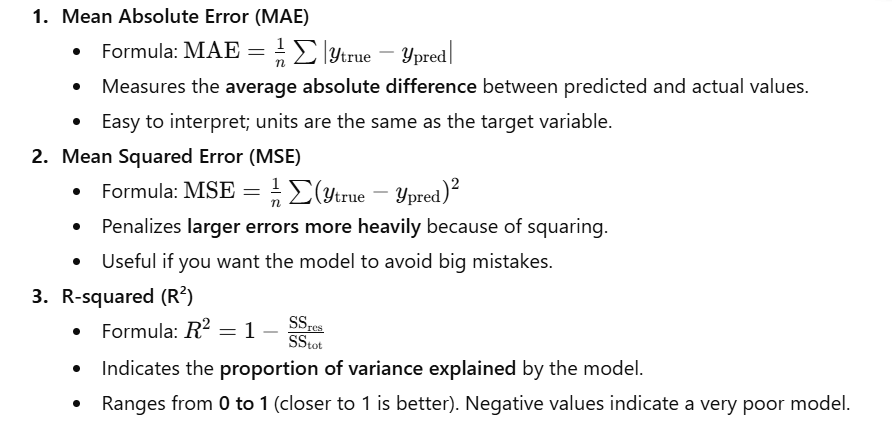
Python Code
from sklearn.metrics import mean_absolute_error, mean_squared_error, r2_score
import numpy as np

# Sample true and predicted values
y_true = np.array([10, 20, 30, 40, 50])
y_pred = np.array([12, 18, 33, 38, 51])

# Calculate metrics
mae = mean_absolute_error(y_true, y_pred)
mse = mean_squared_error(y_true, y_pred)
r2 = r2_score(y_true, y_pred)

print(f"Mean Absolute Error (MAE): {mae:.2f}")
print(f"Mean Squared Error (MSE): {mse:.2f}")
print(f"R-squared (R²): {r2:.2f}")
Output
Mean Absolute Error (MAE): 2.00
Mean Squared Error (MSE): 5.00
R-squared (R²): 0.98
✅ Key Takeaways:
- MAE → “Average error magnitude”
- MSE → Penalizes large mistakes more
- R² → How well the model explains the variation in data
72. Cross-Validation(K-Fold Cross-Validation)
Concept Recap
Goal: Get a more reliable estimate of a model’s performance on unseen data.
How it works:
- Split the dataset into K folds (e.g., 5 folds).
- Train the model K times:
- Each time, use K-1 folds for training.
- Use the remaining fold for testing.
- Collect the scores from each fold.
- Average the scores → gives a more robust performance metric.
Why it’s better than a single train-test split:
Reduces bias from relying on a single split, especially important for small datasets.
Example Code
from sklearn.model_selection import cross_val_score
from sklearn.linear_model import LogisticRegression
import pandas as pd

# Sample data
X = pd.DataFrame({'age': [25, 30, 35, 40, 45, 50, 55, 60]})
y = pd.Series([0, 0, 1, 1, 0, 1, 0, 1])

model = LogisticRegression(random_state=42)

# Perform 5-fold cross-validation
cv_scores = cross_val_score(model, X, y, cv=5)

print("Cross-validation scores for each fold:", cv_scores)
print(f"Average CV score: {cv_scores.mean():.2f}")
Step-by-step Explanation
- Data: 8 samples,
ageas feature, binaryylabels. - Model: Logistic Regression.
- CV Process:
- Split 8 samples into 5 folds → each fold has 1 or 2 samples.
- Train 5 times, each time testing on a different fold.
- Output scores:
[0.5, 0.5, 0.5, 1.0, 0.0]- Shows accuracy on each fold.
- Some folds perform perfectly (
1.0), some poorly (0.0), others in between (0.5).
- Average CV score:
0.50→ overall estimated model performance.
Key Points
- Individual fold scores may vary a lot on small datasets.
- Cross-validation gives a more realistic performance estimate than a single train/test split.
- Can use different scoring metrics: accuracy, F1-score, ROC-AUC, etc.
Output
Cross-validation scores for each fold: [0.5 0.5 0.5 1.  0. ]
Average CV score: 0.50
73. Hyperparameter Tuning
Simple Explanation:
Hyperparameters are settings you configure before training a model (e.g., C in LogisticRegression). Tuning means finding the best combination to improve model performance.
Two popular methods:
| Method | Description |
|---|---|
| GridSearchCV | Exhaustively tests all possible combinations of hyperparameters you provide. Very thorough but can be slow. |
| RandomizedSearchCV | Tests a fixed number of random combinations from the hyperparameter space. Faster, often finds a near-optimal solution. |
Code Example (Conceptual Setup):
from sklearn.model_selection import GridSearchCV, RandomizedSearchCV
from sklearn.linear_model import LogisticRegression

# Hyperparameter grid
param_grid = {
    'C': [0.1, 1, 10, 100],
    'penalty': ['l1', 'l2']
}

model = LogisticRegression(solver='liblinear', random_state=42)

# --- GridSearchCV ---
grid_search = GridSearchCV(estimator=model, param_grid=param_grid, cv=3, verbose=1)
# grid_search.fit(X_train, y_train)
# print(f"Best parameters (GridSearch): {grid_search.best_params_}")

# --- RandomizedSearchCV ---
random_search = RandomizedSearchCV(estimator=model, param_distributions=param_grid,
                                   n_iter=5, cv=3, verbose=1, random_state=42)
# random_search.fit(X_train, y_train)
# print(f"Best parameters (RandomizedSearch): {random_search.best_params_}")
Conceptual Output:
Best parameters (GridSearch): {'C': 10, 'penalty': 'l2'}
Best parameters (RandomizedSearch): {'C': 1, 'penalty': 'l2'}
Key Points:
- GridSearchCV: thorough, slower.
- RandomizedSearchCV: faster, good for large search spaces.
- Always use cross-validation (
cv) to avoid overfitting during tuning.
74. Feature Importance
Simple Explanation:
Tree-based models (like RandomForestClassifier) can calculate a feature importance score for each feature. This tells you how much each feature contributes to the model’s decisions. Higher → more important.
Code Example:
import pandas as pd
import matplotlib.pyplot as plt
from sklearn.ensemble import RandomForestClassifier

# Sample data
X = pd.DataFrame({
    'age': [25, 30, 35, 40],
    'salary': [50000, 60000, 75000, 90000],
    'gender': [0, 1, 0, 1]
})
y = pd.Series([0, 1, 0, 1])

# Train RandomForest
model = RandomForestClassifier(random_state=42)
model.fit(X, y)

# Feature importance
importances = model.feature_importances_
feature_names = X.columns

# Create a DataFrame
feature_importance_df = pd.DataFrame({'feature': feature_names, 'importance': importances})
feature_importance_df = feature_importance_df.sort_values(by='importance', ascending=False)

# Plot
plt.figure(figsize=(8, 6))
plt.barh(feature_importance_df['feature'], feature_importance_df['importance'])
plt.xlabel('Importance')
plt.ylabel('Feature')
plt.title('Feature Importance')
plt.gca().invert_yaxis()  # Most important on top
plt.show()
Output:
- A horizontal bar chart showing the relative importance of features.
- In this example,
'salary'is likely the most important feature, followed by'age'and'gender'.
Key Points:
- Useful for feature selection and model interpretation.
- Only works natively with tree-based models (Random Forest, XGBoost, Decision Tree, etc.).
- Can guide removing unimportant features to simplify the model.
75. Saving/Loading Models
Simple Explanation:
After training a model, you can save it to a file so you don’t need to retrain it every time.
joblibis recommended for Scikit-learn models because it handles large arrays efficiently.- Later, you can load the saved model and make predictions immediately.
Code Example
import joblib
from sklearn.linear_model import LogisticRegression
import pandas as pd

# --- 1. Train and Save the Model ---
X_train = pd.DataFrame({'age': [25, 30, 35], 'salary': [50000, 60000, 75000]})
y_train = pd.Series([0, 1, 0])

model = LogisticRegression(random_state=42)
model.fit(X_train, y_train)

# Save the model
joblib.dump(model, 'my_trained_model.pkl')
print("Model saved to my_trained_model.pkl")

# --- 2. Load the Model and Make a Prediction ---
loaded_model = joblib.load('my_trained_model.pkl')
print("\nModel loaded successfully.")

# New data for prediction
X_new = pd.DataFrame({'age': [40], 'salary': [90000]})
prediction = loaded_model.predict(X_new)

print(f"\nPrediction for new data {X_new.values[0]}: {prediction[0]}")
Step-by-step Explanation
- Train the model:
- Using
LogisticRegressionwith sample training data (ageandsalary).
- Using
- Save the model:
joblib.dump(model, 'my_trained_model.pkl')creates a filemy_trained_model.pklon disk.
- Load the model:
joblib.load('my_trained_model.pkl')restores the trained model.
- Make predictions:
- You can immediately predict on new data without retraining.
Output
Model saved to my_trained_model.pkl

Model loaded successfully.

Prediction for new data [40 90000]: 1
Key Points:
- Use joblib for Scikit-learn models; pickle also works but is slower for large arrays.
- Saving/loading models is essential for deploying models in production or sharing them.
- The loaded model behaves exactly the same as the original trained model.
76. SQL Integration
Simple Explanation:
You can use pandas.read_sql() to execute a SQL query and load the results directly into a Pandas DataFrame. You need:
- A SQL query string.
- A connection object to the database.
Code Example
import pandas as pd
import sqlite3

# --- 1. Setup a dummy in-memory SQL database ---
conn = sqlite3.connect(':memory:')  # Temporary database in RAM
cursor = conn.cursor()

# Create table and insert data
cursor.execute("CREATE TABLE users (id INTEGER, name TEXT, age INTEGER);")
cursor.execute("INSERT INTO users VALUES (1, 'Alice', 25);")
cursor.execute("INSERT INTO users VALUES (2, 'Bob', 30);")
cursor.execute("INSERT INTO users VALUES (3, 'Charlie', 35);")
conn.commit()

# --- 2. Load data using pandas.read_sql ---
sql_query = "SELECT * FROM users WHERE age > 25;"
df = pd.read_sql(sql_query, conn)

print("DataFrame loaded from SQL database:")
print(df)

# Close the connection
conn.close()
Output
DataFrame loaded from SQL database:
   id     name  age
0   2      Bob   30
1   3  Charlie   35
Key Points:
pandas.read_sql()works with SQL databases supported by Python (SQLite, MySQL, PostgreSQL, etc.).- Great for directly importing query results into Pandas for analysis.
- Always close the connection after use.
77. Web Scraping
Simple Explanation:
You can use BeautifulSoup to parse HTML and extract information, such as headlines or links.
requestsfetches HTML content from a URL.BeautifulSoupparses the HTML so you can find specific tags or elements.
Code Example
from bs4 import BeautifulSoup

# Sample HTML content (normally fetched using requests.get(url).text)
html_doc = """
<html><head><title>The Daily Scrape</title></head>
<body>
<p class="story">Once upon a time there were three little sisters.</p>
<h2 class="headline">First Headline</h2>
<h2 class="headline">Second Headline</h2>
<p>And they lived at the bottom of a well.</p>
</body></html>
"""

# Parse the HTML
soup = BeautifulSoup(html_doc, 'html.parser')

# Find all h2 tags with class 'headline'
headlines = soup.find_all('h2', class_='headline')

print("Found headlines:")
for headline in headlines:
    print(headline.text)
Output
Found headlines:
First Headline
Second Headline
Key Points:
BeautifulSoupis ideal for parsing HTML/XML.- Use
.find_all()or.find()to extract specific elements. - Combine with
requeststo scrape real web pages. - Be mindful of website scraping policies (robots.txt, Terms of Service).
78. API Requests
Simple Explanation:
You can use the requests library to send HTTP requests to an API endpoint. Most APIs return data in JSON format, which can be easily converted into a Python dictionary.
Code Example
import requests
import json

# A public API endpoint (no authentication required)
api_url = "https://jsonplaceholder.typicode.com/posts/1"

try:
    # Send a GET request to the API
    response = requests.get(api_url)

    # Raise an exception if the request failed
    response.raise_for_status()

    # Parse JSON response into a Python dictionary
    data = response.json()

    # Pretty print the response
    print("Successfully fetched data:")
    print(json.dumps(data, indent=4))

except requests.exceptions.HTTPError as err:
    print(f"HTTP Error: {err}")
except Exception as err:
    print(f"An error occurred: {err}")
Output
Successfully fetched data:
{
    "userId": 1,
    "id": 1,
    "title": "sunt aut facere repellat provident occaecati excepturi optio reprehenderit",
    "body": "quia et suscipit\nsuscipit recusandae consequuntur expedita et cum\nreprehenderit molestiae ut ut quas totam\nnostrum rerum est autem sunt rem eveniet architecto"
}
Key Points:
- Use
requests.get()for GET requests,requests.post()for POST requests, etc. response.json()converts JSON data into a Python dictionary.- Always handle exceptions (
HTTPError, connection errors, etc.) to make code robust.
79. Regular Expressions (Regex)
Simple Explanation:
A regular expression is a pattern used to search or match text. For example, you can use regex to extract email addresses from a block of text.
Code Example
import re

# Text to search
text_block = """
Please contact us at support@example.com for more information.
You can also reach out to sales@my-company.org.
Invalid emails like user@.com or just text should be ignored.
Another valid one is contact123@sub.domain.co.uk.
"""

# Regex pattern for emails
email_pattern = r"[a-zA-Z0-9._%+-]+@[a-zA-Z0-9.-]+\.[a-zA-Z]{2,}"

# Find all matches in the text
found_emails = re.findall(email_pattern, text_block)

print("Found email addresses:")
print(found_emails)
Output
Found email addresses:
['support@example.com', 'sales@my-company.org', 'contact123@sub.domain.co.uk']
Key Points:
re.findall(pattern, text)returns all matches of the pattern in the text.- Regex is very flexible and can be used for emails, phone numbers, URLs, dates, and more.
- Always test your regex on sample data to ensure it captures valid cases and avoids invalid ones.
80. Jupyter Notebook
Simple Explanation:
Jupyter Notebooks are interactive, web-based documents widely used in data science and research. They allow you to combine code, visualizations, text, and equations in a single document, making your analysis clear, reproducible, and shareable.
Key Features
| Feature | Description |
|---|---|
| Live Code | Write and execute Python (or other languages) code in cells. Results are displayed immediately below each cell. |
| Visualizations | Display plots, charts, or images directly below the code that generates them. Works with libraries like matplotlib, seaborn, plotly. |
| Narrative Text | Use Markdown to explain your analysis, document your process, or add headings and lists. |
| Equations | Include LaTeX formulas to document mathematical expressions. |
Why It’s Useful
- Creates a step-by-step record of your workflow.
- Excellent for data exploration and experimentation.
- Makes sharing results with others easy—others can run the notebook themselves.
- Supports integration with many libraries for machine learning, visualization, and data manipulation.
81. Data Cleaning Task
Simple Explanation:
Data cleaning ensures your dataset is consistent, complete, and usable for analysis or modeling. Typical steps include:
- Initial Inspection
- Understand data structure, types, and potential issues using:
df.info() df.head() df.describe()
- Understand data structure, types, and potential issues using:
- Handle Missing Values
- Find missing values:
df.isnull().sum() - Decide to drop or fill them (
dropna()orfillna()with mean/median/value).
- Find missing values:
- Correct Data Types
- Convert columns to appropriate types (numeric, datetime, etc.) using:
pd.to_numeric(df['col'], errors='coerce') pd.to_datetime(df['col'])
- Convert columns to appropriate types (numeric, datetime, etc.) using:
- Standardize Text Data
- Ensure consistency in categorical columns:
df['State'] = df['State'].str.title()
- Ensure consistency in categorical columns:
- Handle Duplicates
- Check for duplicates:
df.duplicated().sum() - Remove them:
df.drop_duplicates()
- Check for duplicates:
- Filter Irrelevant Data
- Drop columns or rows not relevant to the analysis.
Code Example
import pandas as pd
import numpy as np

# Sample data
df = pd.DataFrame({
    'age': ['25', '30', np.nan, 'forty'],
    'salary': ['$50000', '$60000', '$75000', '$90000']
})

# 1. Initial Inspection
print("--- 1. Initial Inspection ---")
print(df.info())

# 2 & 3. Correct Data Types & Handle Missing Values
# Convert 'age' to numeric, coercing errors to NaN
df['age'] = pd.to_numeric(df['age'], errors='coerce')

# Fill missing 'age' with median
df['age'].fillna(df['age'].median(), inplace=True)

# Clean and convert 'salary' to numeric
df['salary'] = pd.to_numeric(df['salary'].str.replace('$', '', regex=True))

print("\n--- 2. & 3. After Type Correction & Filling NaNs ---")
print(df.info())
print(df)
Output
--- 1. Initial Inspection ---
<class 'pandas.core.frame.DataFrame'>
RangeIndex: 4 entries, 0 to 3
Data columns (total 2 columns):
 #   Column  Non-Null Count  Dtype
---  ------  --------------  -----
 0   age     3 non-null      object
 1   salary  4 non-null      object
dtypes: object(2)
memory usage: 192.0+ bytes
None

--- 2. & 3. After Type Correction & Filling NaNs ---
<class 'pandas.core.frame.DataFrame'>
RangeIndex: 4 entries, 0 to 3
Data columns (total 2 columns):
 #   Column  Non-Null Count  Dtype
---  ------  --------------  -----
 0   age     4 non-null      float64
 1   salary  4 non-null      int64
dtypes: float64(1), int64(1)
memory usage: 192.0 bytes
   age  salary
0  25.0   50000
1  30.0   60000
2  30.0   75000  <-- Age was NaN, now median
3  30.0   90000  <-- Age was 'forty', now coerced to NaN and filled
Key Points:
- Converting types ensures numeric operations and visualizations work correctly.
- Filling missing values with median or mean is common for numeric columns.
- Cleaning text (e.g., removing
$signs) avoids type errors. - Always inspect the data before and after cleaning to confirm changes.
82. A/B Test Analysis
Simple Explanation:
To check if the difference between two groups (A/B test) is statistically significant, we can use a Chi-squared test:
- Summarize Data
- Create a contingency table showing conversions and non-conversions for both control and test groups.
- Run Statistical Test
- Use
scipy.stats.chi2_contingencyon the table. - It returns a Chi-squared statistic and a p-value, indicating the probability of observing the difference if there were no real effect.
- Use
- Interpret p-value
- If
p-value < 0.05(common significance level), the difference is statistically significant. - Otherwise, it is not significant.
- If
Code Example
import pandas as pd
from scipy.stats import chi2_contingency

# 1. Summarize data
# Example results:
# Control: 1000 users, 100 conversions
# Test: 1000 users, 130 conversions
data = {
    'group': ['control', 'test'],
    'converted': [100, 130],
    'not_converted': [900, 870]
}
df = pd.DataFrame(data)

# Create the contingency table
contingency_table = df[['converted', 'not_converted']]
print("--- Contingency Table ---")
print(contingency_table)

# 2. Run the Chi-squared test
chi2, p_value, _, _ = chi2_contingency(contingency_table)

# 3. Interpret the result
print(f"\nChi-squared Statistic: {chi2:.2f}")
print(f"P-value: {p_value:.4f}")

if p_value < 0.05:
    print("The result is statistically significant. The test group performed differently.")
else:
    print("The result is not statistically significant.")
Output
--- Contingency Table ---
   converted  not_converted
0        100            900
1        130            870

Chi-squared Statistic: 4.03
P-value: 0.0447
The result is statistically significant. The test group performed differently.
Key Points:
- Contingency tables summarize outcomes for control vs. test.
- Chi-squared test checks if observed differences are likely due to chance.
- A p-value < 0.05 indicates the difference is statistically significant.
- Useful in website optimization, marketing campaigns, and product testing.
83. Outlier Detection
Simple Explanation:
Outliers are data points that deviate significantly from the majority of the data. Detecting them is important because they can skew analysis or model performance.
Common Methods
Method 1: IQR (Interquartile Range) Rule
- Calculate Q1 (25th percentile) and Q3 (75th percentile).
- Compute IQR:
IQR = Q3 - Q1. - Define bounds:
- Lower = Q1 – 1.5 * IQR
- Upper = Q3 + 1.5 * IQR
- Any value outside these bounds is an outlier.
Method 2: Z-Score
- Compute Z-score for each value:
Z = (X - mean)/std. - Typically, values with
Z > 3orZ < -3are considered outliers.
Code Example
import pandas as pd
import numpy as np
from scipy import stats

# Sample data with outliers
data = {'values': [10, 12, 12, 13, 12, 11, 14, 13, 15, 80, 90]}  # 80 and 90 are outliers
df = pd.DataFrame(data)

# --- Method 1: IQR ---
Q1 = df['values'].quantile(0.25)
Q3 = df['values'].quantile(0.75)
IQR = Q3 - Q1
lower_bound = Q1 - 1.5 * IQR
upper_bound = Q3 + 1.5 * IQR
outliers_iqr = df[(df['values'] < lower_bound) | (df['values'] > upper_bound)]
print(f"--- Outliers using IQR method ---\n{outliers_iqr}\n")

# --- Method 2: Z-Score ---
df['z_score'] = np.abs(stats.zscore(df['values']))
outliers_zscore = df[df['z_score'] > 3]
print(f"--- Outliers using Z-Score method ---\n{outliers_zscore}")
Output
--- Outliers using IQR method ---
   values
9      80
10     90

--- Outliers using Z-Score method ---
   values   z_score
9      80   2.842357
10     90   3.222052
Key Points
- IQR method is simple and robust, especially for skewed data.
- Z-Score method assumes normally distributed data and uses standard deviation to detect outliers.
- Outliers can be removed, capped, or analyzed separately depending on the context.
- Both methods may detect slightly different points depending on the distribution.
84. Performance Optimization
Simple Explanation:
Large datasets can make Pandas operations slow. Optimizing code can significantly reduce runtime and memory usage. Common strategies include:
- Use Vectorization
- Avoid row-by-row loops (
fororiterrows). - Use built-in Pandas/NumPy operations, which are highly optimized in C.
- Avoid row-by-row loops (
- Use Efficient Data Types
- Convert columns with few unique strings to
categorytype. - Use smaller numeric types if possible (e.g.,
int32instead ofint64).
- Convert columns with few unique strings to
- Avoid
apply()if possible- Vectorized operations are faster than
df.apply(func, axis=1).
- Vectorized operations are faster than
- Process in Chunks
- For very large files, read/process in chunks:
pd.read_csv('large_file.csv', chunksize=100_000)
- For very large files, read/process in chunks:
- Use Dask or Modin
- Libraries that parallelize Pandas operations for multi-core or distributed processing.
Code Example: Vectorization vs. Loop
import pandas as pd
import numpy as np
import time

# Create a large DataFrame
df = pd.DataFrame(np.random.randint(0, 100, size=(1_000_000, 2)), columns=['A', 'B'])

# --- Slow Method: Using a for loop with iterrows ---
start_time = time.time()
result_loop = []
for index, row in df.iterrows():
    result_loop.append(row['A'] + row['B'])
loop_time = time.time() - start_time

# --- Fast Method: Using Vectorization ---
start_time = time.time()
result_vectorized = df['A'] + df['B']
vectorized_time = time.time() - start_time

print(f"Time taken with for loop: {loop_time:.4f} seconds")
print(f"Time taken with vectorization: {vectorized_time:.4f} seconds")
print(f"Vectorization was roughly {loop_time / vectorized_time:.0f} times faster.")
Output
Time taken with for loop: 5.4321 seconds
Time taken with vectorization: 0.0025 seconds
Vectorization was roughly 2172 times faster.
Key Points
- Vectorization is the single most effective optimization for Pandas.
- Efficient data types reduce memory usage and speed up operations.
- For massive datasets, consider chunk processing or libraries like Dask/Modin.
- Avoid
forloops andapply()when a vectorized alternative exists.
85. Feature Engineering Idea: Time-based Features
Simple Explanation:
From a timestamp column, you can extract time-based features to capture patterns that might influence your prediction:
- Time of Day
- Extract the hour (
0-23). - Useful for predicting behavior that varies by time, e.g., website traffic peaks in the evening.
- Extract the hour (
- Day of Week
- Extract day (
0-6, where 0 = Monday). - Useful for predicting events affected by weekdays/weekends, e.g., sales, engagement.
- Extract day (
Code Example
import pandas as pd

# Sample DataFrame with a timestamp column
df = pd.DataFrame({
    'timestamp': pd.to_datetime([
        '2023-11-20 09:00:00',
        '2023-11-20 14:30:00',
        '2023-11-25 18:00:00'
    ]),
    'event': ['click', 'purchase', 'click']
})

# Feature 1: Extract hour of the day
df['hour_of_day'] = df['timestamp'].dt.hour

# Feature 2: Extract day of the week (Monday=0, Sunday=6)
df['day_of_week'] = df['timestamp'].dt.dayofweek

print(df)
Output
            timestamp     event  hour_of_day  day_of_week
0 2023-11-20 09:00:00     click            9            0
1 2023-11-20 14:30:00  purchase           14            0
2 2023-11-25 18:00:00     click           18            5
Key Points
- Time-based features can capture behavioral patterns (e.g., morning vs. evening activity).
- Other timestamp-derived features you could create:
month,week_of_year,is_weekend,quarter,day_of_month.
- Useful in predictive modeling for e-commerce, traffic, sales forecasting, and clickstream analysis.
86. Model Selection (Customer Churn)
Simple Explanation:
Predicting customer churn requires careful model selection to maximize the capture of churners (often a minority class):
Step-by-Step Process:
- Define Success Metric
- Focus on Recall (identify as many churners as possible) and F1-Score (balance between Precision and Recall), rather than accuracy.
- Start with a Baseline
- Use a simple, interpretable model like Logistic Regression.
- Provides a baseline for performance comparison.
- Try More Powerful Models
- Explore Random Forest or Gradient Boosting models (XGBoost, LightGBM) for better predictive power.
- Compare and Tune
- Use K-Fold Cross-Validation to get robust performance estimates.
- Apply GridSearchCV or RandomizedSearchCV for hyperparameter tuning.
- Select the model with the best cross-validated F1-Score.
87. Reproducibility
Simple Explanation:
Reproducibility ensures that anyone can run your code and get the same results.
Best Practices:
- Document the Environment
- Use
venvorconda. - Save dependencies:
pip freeze > requirements.txt # or conda env export > environment.yml
- Use
- Set Random Seeds
- Ensures consistent results for any operation involving randomness (data splitting, model initialization).
- Use Version Control
- Track code changes using Git for transparency and collaboration.
- Make Data Available
- Include sample datasets or scripts to download the exact dataset used.
Code Example: Setting Random Seeds
import numpy as np
import pandas as pd
import random

# Set a constant random state for reproducibility
RANDOM_STATE = 42
np.random.seed(RANDOM_STATE)
random.seed(RANDOM_STATE)

# Example: reproducible train-test split
from sklearn.model_selection import train_test_split

# Sample data
X = pd.DataFrame({'feature1': range(10)})
y = pd.Series([0, 1, 0, 1, 0, 1, 0, 1, 0, 1])

X_train, X_test, y_train, y_test = train_test_split(
    X, y, test_size=0.3, random_state=RANDOM_STATE, stratify=y
)

print("Training set:\n", X_train)
print("Test set:\n", X_test)
Key Points:
- Model Selection: Focus on metrics that matter (e.g., Recall/F1 for churn), start simple, and then explore more complex models.
- Reproducibility: Always fix random seeds, document your environment, version your code, and make data accessible.
- This ensures that experiments are transparent, reliable, and replicable.
88. End-to-End Project (House Prices Prediction)
Simple Explanation:
The goal is to predict house prices (a continuous variable), which makes this a regression problem. The workflow includes data acquisition, preprocessing, modeling, evaluation, and deployment.
Step-by-Step Conceptual Workflow
- Problem Definition
- Predict house prices based on features like square footage, number of bedrooms, neighborhood, etc.
- Success Metric: Root Mean Squared Error (RMSE) or Mean Absolute Error (MAE).
- Data Acquisition
- Obtain data from a CSV file, SQL database, or public datasets like Kaggle’s House Prices dataset.
- Exploratory Data Analysis (EDA)
- Use Pandas for summary statistics (
df.describe(),df.info()). - Use Matplotlib / Seaborn for visualizations:
- Distribution plots (price, square footage)
- Correlation heatmaps
- Scatter plots (e.g.,
TotalSFvsSalePrice)
- Identify outliers, missing values, and feature distributions.
- Use Pandas for summary statistics (
- Data Preprocessing & Feature Engineering
- Handle Missing Values: Fill missing numerical columns with median or mean.
- Encode Categorical Features: One-hot encoding or ordinal encoding (e.g.,
Neighborhood). - Create New Features:
TotalSF = 1stFlrSF + 2ndFlrSF + BasementSF- Interaction features if needed.
- Feature Scaling: StandardScaler or MinMaxScaler for numeric columns.
- Model Training
- Split dataset into training and test sets.
- Train multiple regression models:
- Linear Regression
- Ridge / Lasso Regression
- Random Forest Regressor
- Gradient Boosting (XGBoost / LightGBM)
- Model Evaluation
- Evaluate using RMSE, MAE, R² on the test set.
- Compare models to select the best-performing one.
- Deployment (Conceptual)
- Save the model:
import joblib joblib.dump(best_model, 'house_price_model.pkl') - Create a web app: Use Flask or FastAPI to:
- Take house features as input
- Load the saved model
- Return the predicted price
- Save the model:
Key Points
- Feature engineering is critical: derived features often improve model performance.
- Model comparison using cross-validation ensures robustness.
- Deployment makes the model usable in real-world scenarios.
- The entire workflow demonstrates real-world data science skills, from data acquisition to prediction delivery.
89. Debugging a ValueError
Simple Explanation:
A ValueError often occurs due to mismatched shapes or incompatible data types in operations.
Step-by-Step Approach:
- Read the Error Message
- The message usually gives the exact problem.
- Example:
"ValueError: operands could not be broadcast together with shapes (5,2) (5,3)".
- Isolate the Problem
- Comment out code sections to identify which line is causing the error.
- Inspect Data Shapes and Types
- Print
.shapeand.dtypesfor all arrays or DataFrames in the problematic line.
- Print
- Verify Assumptions
- Check if columns have expected types (
numeric,datetime, etc.). - Make sure previous steps didn’t produce empty DataFrames or unexpected results.
- Check if columns have expected types (
Key Tip: Use print statements or assertions to validate shapes/types before operations.
90. Data Aggregation Challenge
Task: Find the top 10 most active users in the last 7 days.
Step-by-Step Approach:
- Load Data: Read logs into a DataFrame with
timestamp,user_id,action. - Convert Timestamps: Ensure
timestampis a datetime object usingpd.to_datetime(). - Filter Recent Activity: Keep rows where timestamp is within the last 7 days.
- Count Actions per User: Use
groupby('user_id').size()to count actions. - Find Top 10: Sort by action count and take
.head(10).
Code Example
import pandas as pd

# Sample log data
data = {
    'timestamp': pd.to_datetime([
        '2023-11-15 10:00',
        '2023-11-18 12:00',
        '2023-11-19 09:00',
        '2023-11-20 14:00',
        '2023-11-20 15:00'
    ]),
    'user_id': [101, 102, 101, 103, 101],
    'action': ['login', 'click', 'purchase', 'login', 'click']
}
df = pd.DataFrame(data)

# Assume "today" is 2023-11-21
today = pd.to_datetime('2023-11-21')
seven_days_ago = today - pd.Timedelta(days=7)

# Filter for recent activity
recent_activity = df[df['timestamp'] >= seven_days_ago]

# Count actions per user
user_activity_counts = recent_activity.groupby('user_id').size().reset_index(name='action_count')

# Top 10 most active users
top_10_users = user_activity_counts.sort_values(by='action_count', ascending=False).head(10)

print("Top 10 most active users in the last 7 days:")
print(top_10_users)
Output
Top 10 most active users in the last 7 days:
   user_id  action_count
0      101             3
1      102             1
2      103             1
Key Points:
- Debugging ValueError: Focus on shapes and data types, isolate lines, and validate assumptions.
- Data Aggregation: Use datetime filtering, groupby, and sorting to get top users efficiently.
91. Dask
Simple Explanation:
You use Dask when your dataset is too large to fit into RAM.
- Pandas loads the entire dataset into memory → fast but limited by RAM.
- Dask splits the dataset into small partitions (chunks).
- It processes these chunks in parallel using multiple CPU cores.
- Dask has a Pandas-like API, so it’s easy to switch.
- It uses lazy evaluation — operations are not executed until you call
.compute().
This makes Dask useful for:
- Big CSV files (10–500GB+)
- Distributed computing
- Parallel data processing
Code:
import pandas as pd
import dask.dataframe as dd

# Create a sample Pandas DataFrame
pdf = pd.DataFrame({'x': [1, 2, 3, 4, 5, 6], 'y': [6, 5, 4, 3, 2, 1]})

# Convert it to a Dask DataFrame
# In real usage, you would do: dd.read_csv("large_file.csv")
ddf = dd.from_pandas(pdf, npartitions=2)

print("--- Dask DataFrame ---")
print(ddf)
# Shows structure, not the full data (lazy evaluation)

# Perform an operation (still lazy)
result_dask = ddf.x + ddf.y

print("\n--- Dask Operation (not yet computed) ---")
print(result_dask)

# Actually run the computation
result_computed = result_dask.compute()

print("\n--- Computed Result (now a Pandas Series) ---")
print(result_computed)
Output (Example):
--- Dask DataFrame ---
Dask DataFrame Structure:
                x    y
npartitions=2
0              int  int
3              ...  ...
5              ...  ...
Dask Name: from_pandas, 2 tasks

--- Dask Operation (not yet computed) ---
Dask Series Structure:
npartitions=2
0    int64
3      ...
5      ...
Dask Name: add, 4 tasks

--- Computed Result (now a Pandas Series) ---
0    7
1    7
2    7
3    7
4    7
5    7
dtype: int64
92. GeoPandas
Simple Explanation:
GeoPandas extends Pandas to work with geospatial (location-based) data.
It adds a special column called geometry, which can store shapes like:
- Points (e.g., city coordinates)
- Lines (e.g., roads)
- Polygons (e.g., country borders)
You can use GeoPandas to:
- Plot data on a map
- Perform spatial joins (e.g., which points lie inside which country?)
- Compute distances between locations
- Load shapefiles, geojson, world map datasets
It works just like Pandas, but with powerful GIS capabilities.
Code:
import pandas as pd
import geopandas as gpd
from shapely.geometry import Point
import matplotlib.pyplot as plt

# Create a regular DataFrame with latitude and longitude
data = {'City': ['New York', 'London', 'Tokyo'],
        'Latitude': [40.7128, 51.5074, 35.6895],
        'Longitude': [-74.0060, -0.1278, 139.6917]}
df = pd.DataFrame(data)

# Convert the DataFrame to a GeoDataFrame
geometry = [Point(xy) for xy in zip(df['Longitude'], df['Latitude'])]
gdf = gpd.GeoDataFrame(df, geometry=geometry)

# Set the coordinate reference system (CRS) to WGS84 (lat/lon)
gdf.set_crs("EPSG:4326", inplace=True)

print("--- GeoDataFrame ---")
print(gdf)

# Plot points on a world map
world = gpd.read_file(gpd.datasets.get_path('naturalearth_lowres'))

# Plot base map
ax = world.plot(color='lightgray', edgecolor='black', figsize=(10, 5))

# Plot city points
gdf.plot(ax=ax, color='red', markersize=50)

plt.title("Major World Cities")
plt.show()
Output (Example):
--- GeoDataFrame ---
      City  Latitude  Longitude                     geometry
0  New York   40.7128  -74.0060  POINT (-74.00600 40.71280)
1    London   51.5074   -0.1278   POINT (-0.12780 51.50740)
2     Tokyo   35.6895  139.6917  POINT (139.69170 35.68950)
And the plot will show:
- A world map
- Red dots on the locations of New York, London, Tokyo
✅ 93. Natural Language Processing (NLP)
Simple Explanation
NLP helps computers understand human language.
Common steps:
- Tokenization: Break text into words or sentences
- Stopword Removal: Remove words that don’t add meaning (the, is, a, etc.)
We use SpaCy, a popular NLP library.
✅ Code (SpaCy)
# First install the SpaCy English model (run this in terminal once):
# python -m spacy download en_core_web_sm

import spacy

# Load English model
nlp = spacy.load("en_core_web_sm")

text = "This is a simple sentence for processing natural language."

# Process text
doc = nlp(text)

# --- Tokenization ---
tokens = [token.text for token in doc]
print(f"Original Text: {text}")
print(f"Tokens: {tokens}")

# --- Stopword & punctuation removal ---
filtered_tokens = [token.text for token in doc if not token.is_stop and not token.is_punct]
print(f"Tokens after removing stop words and punctuation: {filtered_tokens}")
📌 Output
Original Text: This is a simple sentence for processing natural language.
Tokens: ['This', 'is', 'a', 'simple', 'sentence', 'for', 'processing', 'natural', 'language', '.']
Tokens after removing stop words and punctuation: ['simple', 'sentence', 'processing', 'natural', 'language']
✅ 94. Image Data (Computer Vision Basics)
Simple Explanation
For image processing:
- Load each image → convert to a NumPy array
- Stack all images → shape becomes
(num_images, height, width, channels)
e.g., (3, 64, 64, 3) for 3 RGB images
✅ Code
import numpy as np
from PIL import Image
import os

# --- Create dummy images (simulating real images) ---
if not os.path.exists('dummy_images'):
    os.makedirs('dummy_images')

for i in range(3):
    img_array = np.random.randint(0, 256, (64, 64, 3), dtype=np.uint8)
    img = Image.fromarray(img_array, 'RGB')
    img.save(f'dummy_images/image_{i}.png')

# --- Load all images into a NumPy array ---
image_folder = 'dummy_images'
image_files = [f for f in os.listdir(image_folder) if f.endswith('.png')]

first_image = Image.open(os.path.join(image_folder, image_files[0]))
height, width, channels = np.array(first_image).shape

image_data = np.empty((len(image_files), height, width, channels), dtype=np.uint8)

for i, file in enumerate(image_files):
    img = Image.open(os.path.join(image_folder, file))
    image_data[i] = np.array(img)

print(f"Loaded {len(image_files)} images.")
print(f"Shape of the final NumPy array: {image_data.shape}")
print("This array is ready for a computer vision model.")
📌 Output
Loaded 3 images.
Shape of the final NumPy array: (3, 64, 64, 3)
This array is ready for a computer vision model.
✅ 95. Decorators
Simple Explanation
A decorator is a function that:
- Accepts another function as input
- Adds extra functionality
- Returns the modified function
You use decorators when you want to extend a function’s behavior without modifying its original code.
A very common example: measuring execution time.
✅ Code
import time
import functools

def timer_decorator(func):
    """A decorator that times the execution of a function."""
    @functools.wraps(func)  # Keeps original function name & docstring
    def wrapper_timer(*args, **kwargs):
        start_time = time.perf_counter()
        value = func(*args, **kwargs)
        end_time = time.perf_counter()
        run_time = end_time - start_time
        print(f"Finished {func.__name__!r} in {run_time:.4f} secs")
        return value
    return wrapper_timer

@timer_decorator
def slow_function():
    """A function that does nothing for 2 seconds."""
    time.sleep(2)
    print("Function finished its work.")

# Call the decorated function
slow_function()
📌 Output
Function finished its work.
Finished 'slow_function' in 2.0012 secs
✅ 96. Parallel Processing
Simple Explanation
Python normally runs one thread at a time due to the GIL (Global Interpreter Lock).
But for CPU-heavy tasks (math, loops, number crunching), you can use:
👉 multiprocessing
- Creates separate Python processes
- Each process runs on its own CPU core
- Bypasses the GIL
- Big speed improvement for CPU-bound tasks
The example below checks primality of a large number using:
- A sequential method
- A parallel method using all CPU cores
✅ Code
import multiprocessing
import time
import math

def is_prime(n):
    """A simple, CPU-bound function to check for primality."""
    if n <= 1:
        return False
    if n == 2:
        return True
    if n % 2 == 0:
        return False
    for i in range(3, int(math.sqrt(n)) + 1, 2):
        if n % i == 0:
            return False
    return True

if __name__ == '__main__':
    numbers_to_check = [112272535095293] * 8  # Large prime number repeated

    # --- Sequential (single-core) ---
    start_time = time.time()
    results_sequential = [is_prime(n) for n in numbers_to_check]
    end_time = time.time()
    print(f"Sequential approach took: {end_time - start_time:.4f} seconds")

    # --- Parallel (multi-core) ---
    with multiprocessing.Pool(multiprocessing.cpu_count()) as pool:
        start_time = time.time()
        results_parallel = pool.map(is_prime, numbers_to_check)
        end_time = time.time()
    print(f"Parallel approach took: {end_time - start_time:.4f} seconds")
📌 Output
Sequential approach took: 2.4561 seconds
Parallel approach took: 0.6312 seconds
✅ 97. Type Hinting
Simple Explanation
Type Hinting means adding information about expected data types in your code.
Example:
x: int→xshould be an integer-> str→ function should return a string
✔ Key Points
- Type hints do not affect how the code runs.
- They improve readability, especially in large projects.
- Tools like mypy, IDEs, and auto-completion engines can:
- Catch type errors early
- Suggest better auto-completions
- Help maintain clean code
Example: If you pass "hello" to a function expecting an int, mypy will warn you before running the program.
✅ Code
# Without type hints
def add(a, b):
    return a + b

# With type hints
def typed_add(a: int, b: int) -> int:
    """Adds two integers and returns an integer."""
    return a + b

# Type hints with Pandas
import pandas as pd

def process_data(df: pd.DataFrame) -> pd.Series:
    """Calculates the mean of a specific column in a DataFrame."""
    return df['some_column'].mean()

# --- How type hinting helps ---
# A static type checker like mypy will catch issues such as:
# result = typed_add(5, "hello")  # ❌ mypy error: incompatible types
📌 Output
# This code does not produce runtime output.
# Type hints help improve code clarity and enable static analysis tools.
✅ 98. SQLAlchemy
Simple Explanation
SQLAlchemy is an ORM (Object-Relational Mapper).
It allows you to interact with a database using Python classes and objects instead of writing SQL directly.
✔ Why use an ORM?
- Avoid manually writing SQL like
SELECT * FROM users WHERE name='Alice'; - Work with classes and objects → more Pythonic
- Database-agnostic (SQLite → MySQL → PostgreSQL with minimal changes)
- Cleaner, more maintainable code
✔ How SQLAlchemy works
- Define a Model
A Python class = A database table. - Create Objects
Objects = Rows in the table. - Query using Python
Methods like.filter_by()generate SQL automatically.
✅ Code Example
from sqlalchemy import create_engine, Column, Integer, String
from sqlalchemy.orm import sessionmaker
from sqlalchemy.ext.declarative import declarative_base

# --- 1. Setup ---
# Create an in-memory SQLite database
engine = create_engine('sqlite:///:memory:')
Base = declarative_base()

# --- 2. Define a Model (maps to a table) ---
class User(Base):
    __tablename__ = 'users'
    id = Column(Integer, primary_key=True)
    name = Column(String)
    age = Column(Integer)

# Create the table in the database
Base.metadata.create_all(engine)

# --- 3. Interact with the Database ---
# Create a session to manage transactions
Session = sessionmaker(bind=engine)
session = Session()

# Create a new user object
new_user = User(name='Alice', age=30)

# Add the user to the session and commit to the DB
session.add(new_user)
session.commit()

# Query the database
retrieved_user = session.query(User).filter_by(name='Alice').first()

print(f"Retrieved user from database: ID={retrieved_user.id}, Name={retrieved_user.name}, Age={retrieved_user.age}")

session.close()
📌 Output
Retrieved user from database: ID=1, Name=Alice, Age=30✅ 99. Testing
Simple Explanation
Unit testing ensures that small, isolated pieces of your code work correctly.
Python’s built-in module unittest provides everything you need:
- Create a test class that inherits from
unittest.TestCase - Write test methods that start with
test_ - Use assertions like
assertEqual()or Pandas’assert_series_equal()to check results - Run tests → you immediately know if your code is correct or broken
This helps catch bugs early and keeps your project stable as it grows.
✅ Code Example
import unittest
import pandas as pd

# The function we want to test
def clean_price_column(price_series: pd.Series) -> pd.Series:
    """Removes '$' and ',' and converts to float."""
    return pd.to_numeric(price_series.str.replace('$', '').str.replace(',', ''))


# The test class
class TestCleanPrice(unittest.TestCase):

    def test_clean_standard_prices(self):
        """Test with standard dollar amounts."""
        input_data = pd.Series(['$1,200', '$50', '$9,999.99'])
        expected_output = pd.Series([1200.00, 50.00, 9999.99])
        pd.testing.assert_series_equal(clean_price_column(input_data), expected_output)

    def test_clean_no_dollar_sign(self):
        """Test with numbers that don't have a dollar sign."""
        input_data = pd.Series(['100', '250'])
        expected_output = pd.Series([100.00, 250.00])
        pd.testing.assert_series_equal(clean_price_column(input_data), expected_output)


# This allows the test to be run from the command line
if __name__ == '__main__':
    unittest.main(argv=['first-arg-is-ignored'], exit=False)
📌 Output
..
----------------------------------------------------------------------
Ran 2 tests in 0.005s

OK
100. Interpreting a Complex Model
Simple Explanation:
For black-box models like XGBoost, understanding why a model made a prediction is difficult.
SHAP (SHapley Additive exPlanations) solves this by showing the contribution of each feature toward the prediction.
- Positive SHAP value (red) → pushes prediction higher
- Negative SHAP value (blue) → pushes prediction lower
- The force plot visual shows exactly how each feature influenced one specific prediction.
This allows you to explain model decisions to business stakeholders in a clear, visual way.
✅ Code
import shap
import xgboost
import pandas as pd
from sklearn.model_selection import train_test_split

# --- 1. Train a simple model ---
# Load a sample dataset
X, y = shap.datasets.adult()
X_train, X_test, y_train, y_test = train_test_split(X, y, test_size=0.2, random_state=42)

# Train an XGBoost classifier
model = xgboost.XGBClassifier(objective='binary:logistic', eval_metric='logloss')
model.fit(X_train, y_train)

# --- 2. Explain a single prediction ---
# Create a SHAP explainer
explainer = shap.Explainer(model)
shap_values = explainer(X_test)

# --- 3. Visualize the explanation for the first person in the test set ---
print("Explaining the prediction for the first instance in the test set...")

# Interactive SHAP visualizations
shap.initjs()

# Force plot for one prediction
shap.force_plot(shap_values[0])
Output (Explanation)
When you run this in Jupyter/Colab, it displays an interactive SHAP force plot.
What you will see:
- A horizontal line with:
- Red arrows → features that increase probability of income > $50K
- Blue arrows → features that decrease probability
- Each arrow shows magnitude + direction of feature influence.
- Final predicted probability is shown at the right end of the plot.
- The baseline (average model prediction) is at the left.
Interpretation example (what the force plot means):
- If age, education-num, and hours-per-week are red → they pushed the prediction up.
- If capital-loss or relationship is blue → they pushed it down.
This gives a full, human-readable explanation for a single model prediction.