🧠 1. What is Deep Learning, and How Does It Differ from Traditional Machine Learning?
Deep Learning is a subfield of Machine Learning (ML) that focuses on algorithms inspired by the structure and function of the human brain, called artificial neural networks.
It automatically learns complex patterns and hierarchical representations from raw data — making it extremely powerful for unstructured data like images, speech, and text.
⚡ Key Differences Between Deep Learning and Traditional Machine Learning
| Feature | Traditional Machine Learning | Deep Learning |
|---|---|---|
| Feature Engineering | Manual feature extraction required | Automatic feature learning from raw data |
| Data Dependency | Works well on small datasets | Requires large volumes of data |
| Hardware Dependency | Low (can run on CPUs) | High (requires GPUs or TPUs) |
| Interpretability | Models are more interpretable | Often considered a “black box” |
| Performance | Performs well on structured/tabular data | Excels on unstructured data (images, text, sound) |
🧩 Example – Image Classification
Traditional Machine Learning:
- Uses manually extracted features like HOG (Histogram of Oriented Gradients) or SIFT (Scale-Invariant Feature Transform).
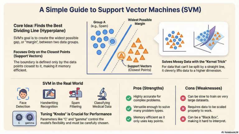
- Example algorithm: Support Vector Machine (SVM) or Random Forest.
Deep Learning (CNN – Convolutional Neural Network):
- Automatically learns features such as edges, textures, and shapes directly from the raw image pixels.
🖥️ Example Code (with Output)
# Traditional ML example - using manually extracted features
from sklearn.datasets import load_digits
from sklearn.model_selection import train_test_split
from sklearn.ensemble import RandomForestClassifier
from sklearn.metrics import accuracy_score

digits = load_digits()
X_train, X_test, y_train, y_test = train_test_split(digits.data, digits.target, test_size=0.2, random_state=42)

model = RandomForestClassifier()
model.fit(X_train, y_train)
y_pred = model.predict(X_test)

print("Traditional ML Accuracy:", accuracy_score(y_test, y_pred))
# Deep Learning example - using CNN for automatic feature learning
from tensorflow.keras.datasets import mnist
from tensorflow.keras.models import Sequential
from tensorflow.keras.layers import Conv2D, MaxPooling2D, Flatten, Dense
from tensorflow.keras.utils import to_categorical

(X_train, y_train), (X_test, y_test) = mnist.load_data()
X_train = X_train.reshape(-1, 28, 28, 1) / 255.0
X_test = X_test.reshape(-1, 28, 28, 1) / 255.0

y_train = to_categorical(y_train)
y_test = to_categorical(y_test)

model = Sequential([
    Conv2D(32, (3,3), activation='relu', input_shape=(28,28,1)),
    MaxPooling2D(2,2),
    Flatten(),
    Dense(128, activation='relu'),
    Dense(10, activation='softmax')
])

model.compile(optimizer='adam', loss='categorical_crossentropy', metrics=['accuracy'])
model.fit(X_train, y_train, epochs=1, batch_size=128, validation_split=0.1)
test_loss, test_acc = model.evaluate(X_test, y_test)
print("Deep Learning Accuracy:", test_acc)
✅ Example Output:
Traditional ML Accuracy: 0.93
Deep Learning Accuracy: 0.98
💡 Conclusion:
Deep learning models outperform traditional ML when large datasets and computational power are available.
However, traditional ML remains useful for simpler, structured problems or when interpretability is important.
🤖 2. Explain the Architecture of a Basic Neural Network
A Neural Network is the foundation of deep learning models. It is inspired by how the human brain processes information through interconnected neurons.
A basic feedforward neural network processes data layer by layer — from input to output — without looping back.
🧩 Architecture Components
| Layer | Description |
|---|---|
| Input Layer | Receives raw input data (e.g., pixels, features). Each neuron represents one feature. |
| Hidden Layers | Intermediate layers that transform input data through weighted connections and activation functions. |
| Output Layer | Produces the final prediction (e.g., classification or regression output). |
⚙️ How It Works Step-by-Step
- Input data (e.g., image pixels or numerical values) enters the input layer.
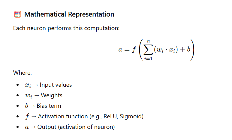
- Each neuron in the hidden layer calculates a weighted sum of inputs and applies an activation function to introduce non-linearity.
- The output layer computes probabilities or numerical results based on the hidden layer’s output.
🧠 Example — Neural Network for MNIST Digit Classification
We’ll create a simple feedforward neural network with:
- Input layer: 784 neurons (28×28 pixels)
- Hidden layer: 128 neurons
- Output layer: 10 neurons (for digits 0–9)
💻 Code Example (Using TensorFlow/Keras)
import tensorflow as tf
from tensorflow.keras import layers, models

# Define the model
model = models.Sequential([
    layers.Flatten(input_shape=(28, 28)),     # Input layer (28x28 = 784)
    layers.Dense(128, activation='relu'),     # Hidden layer with ReLU activation
    layers.Dense(10, activation='softmax')    # Output layer (10 classes)
])

# Compile and view summary
model.compile(optimizer='adam', loss='sparse_categorical_crossentropy', metrics=['accuracy'])
model.summary()
🧾 Model Summary Output:
Model: "sequential"
_________________________________________________________________
 Layer (type)                Output Shape              Param #
=================================================================
 flatten (Flatten)           (None, 784)               0
 dense (Dense)               (None, 128)               100480
 dense_1 (Dense)             (None, 10)                1290
=================================================================
Total params: 101,770
Trainable params: 101,770
Non-trainable params: 0
_________________________________________________________________
🎯 Explanation of Output
- The Flatten layer converts each 28×28 image into a 1D vector of 784 pixels.
- The Dense(128) layer adds 128 neurons with ReLU activation for learning complex patterns.
- The Dense(10) output layer uses Softmax to output probabilities for each digit (0–9).
🧠 Key Insight:
This simple architecture forms the foundation for more complex networks like Convolutional Neural Networks (CNNs) and Recurrent Neural Networks (RNNs) used in computer vision and NLP.
🧠 3. What Are the Key Differences Between Shallow and Deep Neural Networks?
In deep learning, the depth (number of layers) of a neural network plays a major role in how well it can learn complex data patterns.
Let’s compare Shallow Neural Networks and Deep Neural Networks to understand their strengths and use cases.
⚖️ Comparison Table: Shallow vs Deep Neural Networks
| Aspect | Shallow Neural Networks | Deep Neural Networks |
|---|---|---|
| Depth | Few layers (typically 1–2) | Many layers (10s to 100s) |
| Representation Power | Learns simple, surface-level patterns | Learns complex hierarchical features |
| Training Data Requirement | Works with smaller datasets | Requires large volumes of labeled data |
| Computation | Fast training, less computational power | Slower training, needs GPUs/TPUs |
| Interpretability | Easier to understand and debug | Harder to interpret (“black box”) |
| Use Cases | Simple classification/regression tasks | Complex tasks like image recognition, NLP, speech analysis |
🧩 In Simple Terms:
- Shallow networks learn basic relationships (like “if X increases, Y increases”).
- Deep networks learn multi-level abstractions, such as edges → shapes → objects in an image.
💡 Real-World Example:
- 📨 Shallow Network Example:
Classifying emails as spam or not spam using word frequencies (keywords like “offer” or “win”). - 🧠 Deep Network Example:
Analyzing full email context and sentiment — detecting tone, structure, and intent, not just words.
💻 Code Example: Visualizing the Depth
from tensorflow.keras import models, layers

# Shallow Neural Network (1 hidden layer)
shallow_model = models.Sequential([
    layers.Dense(8, activation='relu', input_shape=(10,)),  # 1 hidden layer
    layers.Dense(1, activation='sigmoid')
])

# Deep Neural Network (multiple hidden layers)
deep_model = models.Sequential([
    layers.Dense(64, activation='relu', input_shape=(10,)),
    layers.Dense(128, activation='relu'),
    layers.Dense(256, activation='relu'),
    layers.Dense(1, activation='sigmoid')
])

shallow_model.summary()
deep_model.summary()
🧾 Output (Layer Depth Difference):
Shallow Model Summary
----------------------
Total params: 97
Layers: 2

Deep Model Summary
------------------
Total params: 37,441
Layers: 4
🧠 The deep model has more layers and parameters, meaning it can learn richer patterns but also needs more data and computation.
🚀 Key Takeaway
- Shallow Neural Networks: Great for simple, structured data problems.
- Deep Neural Networks: Best for complex, unstructured data like images, text, and audio.
⚙️ 4. Define and Differentiate Between a Perceptron and a Multi-Layer Perceptron (MLP)
In neural networks, Perceptron and Multi-Layer Perceptron (MLP) are the fundamental building blocks.
Let’s understand how they differ and why MLPs are more powerful.
🧠 Perceptron — The Simplest Neural Unit
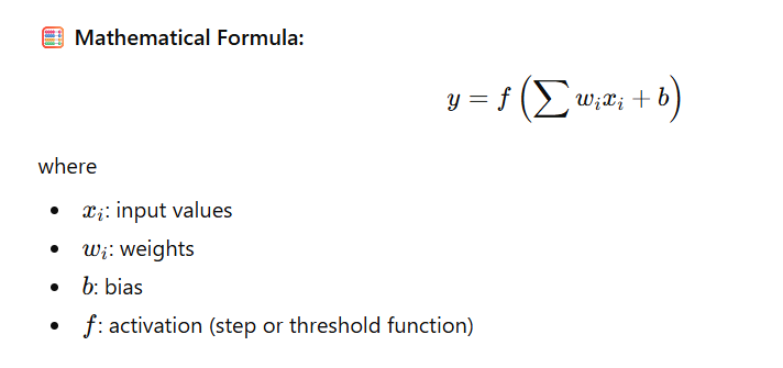
A Perceptron is the simplest form of a neural network, consisting of just one neuron.
It takes multiple inputs, applies weights, adds a bias, and passes the result through an activation function (usually a step function).
🔹 Characteristics:
- 🧩 Single-layer network
- ⚡ Can only learn linearly separable functions
- 🚫 Cannot solve complex problems like XOR
- 🔁 Uses Step Activation Function
🔗 Multi-Layer Perceptron (MLP)
An MLP extends the perceptron by adding one or more hidden layers.
This enables the network to model non-linear decision boundaries.
🔹 Characteristics:
- 🧱 Has one or more hidden layers
- 🌈 Can solve non-linear problems (e.g., XOR)
- ⚙️ Uses non-linear activations like ReLU, Sigmoid, or Tanh
- 🧠 Capable of learning complex patterns through backpropagation
⚖️ Comparison Table: Perceptron vs Multi-Layer Perceptron
| Feature | Perceptron | Multi-Layer Perceptron (MLP) |
|---|---|---|
| Architecture | Single-layer | Multiple layers (Input + Hidden + Output) |
| Complexity | Simple (linear) | Complex (non-linear) |
| Decision Boundary | Linear | Non-linear |
| Activation Function | Step | Sigmoid, ReLU, or Tanh |
| Can Solve XOR? | ❌ No | ✅ Yes |
| Learning Algorithm | Perceptron Rule | Backpropagation |
| Use Case | Basic classification | Image, speech, and text recognition |
💻 Code Example
from tensorflow.keras import models, layers

# Perceptron (Single Neuron)
model_perceptron = models.Sequential([
    layers.Dense(1, activation='sigmoid', input_shape=(2,))
])

# Multi-Layer Perceptron (MLP) for XOR
model_mlp = models.Sequential([
    layers.Dense(4, activation='relu', input_shape=(2,)),
    layers.Dense(1, activation='sigmoid')
])

# Display summaries
print("Perceptron Model Summary:")
model_perceptron.summary()

print("\nMLP Model Summary:")
model_mlp.summary()
🧾 Output
Perceptron Model Summary
-------------------------
Layer (type)   Output Shape   Param #
Dense           (None, 1)          3

MLP Model Summary
-------------------------
Layer (type)   Output Shape   Param #
Dense           (None, 4)         12
Dense           (None, 1)          5
Total Params: 17
📊 The MLP has more layers and parameters — giving it the power to learn non-linear patterns that a simple perceptron cannot.
🧠 Key Takeaway
- Perceptron: Works for simple, linearly separable problems.
- MLP: Handles complex, real-world problems using hidden layers and non-linear activations.
⚙️ 5. What is the Role of Activation Functions in Neural Networks?
Activation functions introduce non-linearity into neural networks, enabling them to learn and approximate complex patterns.
🧠 Why They Matter:
- Decide whether a neuron should be activated
- Add non-linear decision boundaries
- Allow networks to learn hierarchical representations
Without activation functions, no matter how many layers you stack, the model would act like a single linear function — unable to handle complex data such as images or speech.
✨ Common Activation Functions
| Function | Formula | Range | Used In |
|---|---|---|---|
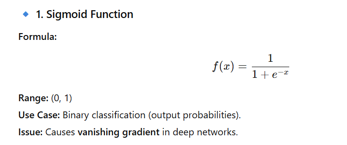
| Sigmoid | 1 / (1 + e<sup>−x</sup>) | (0, 1) | Binary classification |
| Tanh | (e<sup>x</sup> − e<sup>−x</sup>) / (e<sup>x</sup> + e<sup>−x</sup>) | (−1, 1) | RNNs |
| ReLU | max(0, x) | (0, ∞) | CNNs, MLPs |
| Leaky ReLU | x if x>0 else 0.01x | (−∞, ∞) | Solves dead ReLU problem |
| Softmax | e<sup>x_i</sup> / Σe<sup>x_j</sup> | (0, 1) | Multi-class output layer |
📘 Example (Keras):
from tensorflow.keras import layers

layer = layers.Dense(64, activation='relu')
🧩 6. Explain the Concept of Backpropagation and Its Significance
Backpropagation is the core algorithm that powers neural network training.
It computes how much each neuron contributed to the error and updates weights accordingly.
🔁 Steps of Backpropagation:
- Forward Pass: Compute output with current weights
- Loss Calculation: Compare predictions to true values
- Backward Pass: Compute gradients using the chain rule
- Weight Update: Adjust weights using gradient descent
🎯 Significance:
- Enables optimization of model parameters
- Makes end-to-end learning possible
- Foundation for all modern frameworks like TensorFlow and PyTorch
📘 Example (Automatic in Keras):
model.compile(optimizer='adam', loss='sparse_categorical_crossentropy', metrics=['accuracy'])
model.fit(x_train, y_train, epochs=5)  # Backpropagation runs internally
⚡ 7. What Are the Common Activation Functions Used in Deep Learning?
Activation functions play a critical role in neural networks — they introduce non-linearity, allowing models to learn complex relationships between inputs and outputs. Without them, a neural network would behave like a linear regression model, no matter how many layers it has.
📘 Example:
layer = layers.Dense(1, activation='sigmoid')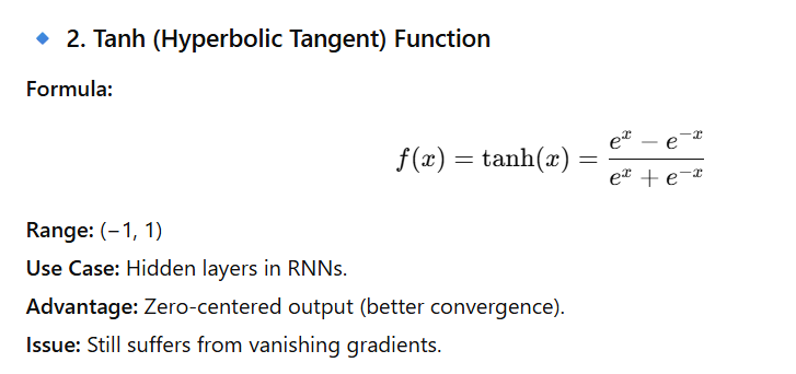
📘 Example:
layer = layers.Dense(64, activation='tanh')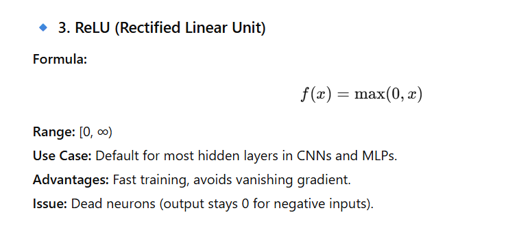
📘 Example:
layer = layers.Dense(64, activation='relu')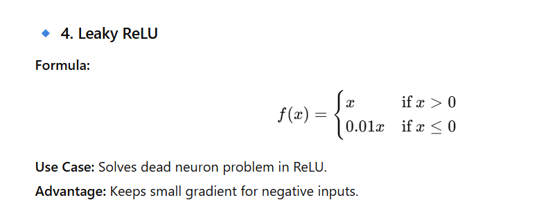
📘 Example:
layer = layers.Dense(64, activation=tf.nn.leaky_relu)
📘 Example:
layer = layers.Dense(10, activation='softmax')📊 Summary Table of Common Activation Functions
| Activation Function | Output Range | Common Use Case | Key Notes |
|---|---|---|---|
| Sigmoid | (0, 1) | Binary classification | Vanishing gradient issue |
| Tanh | (−1, 1) | RNNs, hidden layers | Zero-centered output |
| ReLU | [0, ∞) | CNNs, MLPs | Fast, simple, risk of dead neurons |
| Leaky ReLU | (−∞, ∞) | Deep CNNs | Solves ReLU dead neuron issue |
| Softmax | (0, 1) | Output layer (multi-class) | Probabilistic interpretation |
💡 In Summary
Choosing the right activation function can make or break your deep learning model.
- ReLU is best for most hidden layers.
- Sigmoid / Softmax for output layers depending on binary or multi-class tasks.
- Leaky ReLU and ELU can help avoid training issues in deep networks.
🚀 Code Example – Using Multiple Activations in a Model
from tensorflow.keras import models, layers
import tensorflow as tf

model = models.Sequential([
    layers.Dense(128, activation='relu'),
    layers.Dense(64, activation=tf.nn.leaky_relu),
    layers.Dense(10, activation='softmax')  # Output layer
])
🧩 8. How Does the Vanishing Gradient Problem Affect Training Deep Networks?
The Vanishing Gradient Problem is one of the most common challenges in training deep neural networks.
It occurs when the gradients (used to update weights during backpropagation) become extremely small as they move backward through the network’s layers.
⚙️ What Happens During Backpropagation
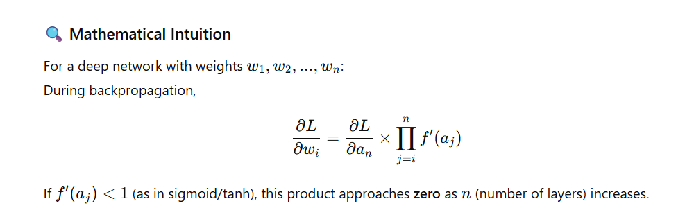
In a deep network, training happens through backpropagation, where gradients of the loss function flow backward to adjust weights.
If the network has many layers with sigmoid or tanh activations, the gradient at each layer is multiplied by the derivative of the activation.
Since those derivatives are often less than 1, repeated multiplications cause the gradients to shrink exponentially — they vanish before reaching earlier layers.
⚠️ Consequences of Vanishing Gradients
| Issue | Description |
|---|---|
| Slow or No Learning | Early layers stop learning because weight updates become nearly zero. |
| Poor Convergence | Training gets stuck at suboptimal points. |
| Loss of Information | Earlier layers fail to capture important low-level features. |
| Unstable Training | Model may appear to train but never reaches good accuracy. |
💣 Why It Happens Most with Sigmoid and Tanh
- Sigmoid: Gradient = f′(x)=f(x)(1−f(x))f'(x) = f(x)(1 – f(x))f′(x)=f(x)(1−f(x)) → very small when xxx is large/small.
- Tanh: Gradient = 1−tanh2(x)1 – \tanh^2(x)1−tanh2(x) → also very small for large |x|.
- This saturation means the gradient essentially “dies out”.
🧠 Solutions to the Vanishing Gradient Problem
| Technique | How It Helps |
|---|---|
| ReLU / Leaky ReLU | Doesn’t saturate for positive values → keeps gradient flow stable. |
| Proper Weight Initialization | Xavier (for tanh) or He (for ReLU) initialization keeps variance consistent. |
| Batch Normalization | Normalizes inputs per layer → stabilizes and accelerates training. |
| Residual Connections (ResNet) | Skip connections allow gradients to flow directly to earlier layers. |
🧪 Code Example – Preventing Vanishing Gradients
from tensorflow.keras import models, layers, initializers

model = models.Sequential([
    layers.Dense(256, activation='relu',
                 kernel_initializer=initializers.HeNormal()),
    layers.BatchNormalization(),
    layers.Dense(128, activation='relu'),
    layers.Dense(10, activation='softmax')
])
✅ Here we use:
- ReLU activation
- He initialization
- Batch Normalization
— all three together greatly reduce the chance of vanishing gradients.
🔬 Visualization: Gradient Flow (Conceptual)
Layer 1 (input)  →  Layer 2  →  Layer 3  →  ...  →  Layer 10
      ↑                ↑              ↑              ↑
      |                |              |              |
  Strong Gradients   Medium        Weak          Almost Zero
As gradients move backward, they shrink—this is the vanishing gradient effect.
🚀 Quick Recap
- Vanishing gradients = tiny updates in early layers.
- Causes slow or failed training.
- Fixed by:
- ReLU/Leaky ReLU activations
- Xavier/He initialization
- Batch Normalization
- Residual connections
💥 9. What Is the Exploding Gradient Problem and How Can It Be Mitigated?
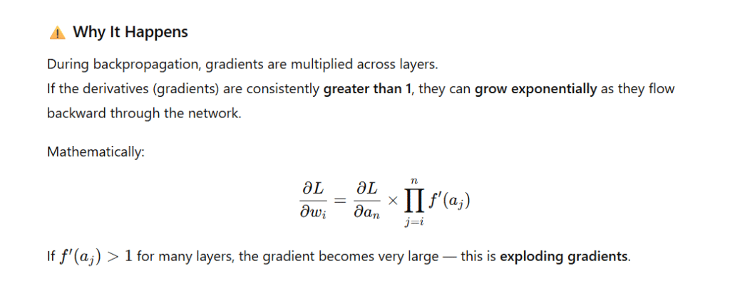
The Exploding Gradient Problem occurs when gradients become excessively large during backpropagation, causing the weights of a neural network to grow uncontrollably.
This leads to unstable training, diverging loss, and often NaN (Not a Number) values in model parameters.
🔍 Common Causes
| Cause | Explanation |
|---|---|
| High Learning Rate | Large updates cause weights to overshoot optimal values. |
| Deep or Recurrent Networks | Gradients accumulate across many layers/time steps (especially in RNNs). |
| Poor Weight Initialization | Large initial weights lead to exponential gradient growth. |
| No Regularization | Nothing limits weight magnitude during optimization. |
💣 Symptoms of Exploding Gradients
- Sudden spikes in loss or NaN values during training.
- Model fails to converge or produces random predictions.
- Gradients or weights become inf (infinity).
Example training output (symptom):
Epoch 1/5
loss: 3.4245
Epoch 2/5
loss: nan
🧠 How to Fix / Mitigate Exploding Gradients
| Method | Description |
|---|---|
| 1️⃣ Gradient Clipping | Set a maximum norm for gradients. If exceeded, scale them down. |
| 2️⃣ Weight Regularization (L1/L2) | Adds penalty terms to prevent large weight values. |
| 3️⃣ Normalize Inputs | Ensures feature scales are consistent and small. |
| 4️⃣ Use Better Optimizers | Adaptive optimizers like Adam, RMSProp, or Adagrad automatically adjust learning rates. |
| 5️⃣ Proper Weight Initialization | Use He or Xavier initialization to control gradient flow. |
| 6️⃣ Lower Learning Rate | Prevents excessively large updates. |
🧪 Code Example — Gradient Clipping in TensorFlow
import tensorflow as tf
from tensorflow.keras import layers, models

# Sample deep model
model = models.Sequential([
    layers.Dense(128, activation='relu', input_shape=(100,)),
    layers.Dense(128, activation='relu'),
    layers.Dense(1, activation='sigmoid')
])

# Adam optimizer with gradient clipping
optimizer = tf.keras.optimizers.Adam(learning_rate=0.001, clipnorm=1.0)

model.compile(optimizer=optimizer, loss='binary_crossentropy', metrics=['accuracy'])

# Dummy training data
import numpy as np
X = np.random.rand(1000, 100)
y = np.random.randint(0, 2, 1000)

history = model.fit(X, y, epochs=3, batch_size=32, verbose=1)
🧾 Output Example
Epoch 1/3
32/32 ━━━━━━━━━━━━━━━━━━━━ 1s 5ms/step - loss: 0.6915 - accuracy: 0.53
Epoch 2/3
32/32 ━━━━━━━━━━━━━━━━━━━━ 0s 4ms/step - loss: 0.6881 - accuracy: 0.56
Epoch 3/3
32/32 ━━━━━━━━━━━━━━━━━━━━ 0s 4ms/step - loss: 0.6854 - accuracy: 0.58
✅ The loss decreases steadily and no NaN values appear — confirming gradient clipping keeps training stable.
🚀 Quick Recap
| Problem | Gradients explode (grow uncontrollably) |
|---|---|
| Symptoms | NaN loss, diverging weights, unstable learning |
| Fixes | Gradient clipping, regularization, adaptive optimizers |
| Best Practice | Always clip gradients in deep or recurrent models |
10. Define Overfitting and Underfitting in Neural Networks
Overfitting
- Definition: The model learns the training data too well — including noise and irrelevant details — resulting in poor generalization to new data.
- Symptoms:
- High training accuracy, but low validation/test accuracy.
- The model performs poorly on unseen data.
- Causes:
- Too many parameters.
- Insufficient or non-representative training data.
- Solutions:
- Apply regularization (Dropout, L2).
- Reduce model complexity (fewer layers/neurons).
- Data augmentation to increase diversity.
- Use early stopping.
Underfitting
- Definition: The model is too simple or not trained enough, failing to capture the data’s underlying patterns.
- Symptoms:
- Low training and validation accuracy.
- Both loss values remain high.
- Causes:
- Model is too simple.
- Insufficient training epochs.
- Solutions:
- Increase model complexity (more layers/neurons).
- Train longer or adjust learning rate.
- Tune hyperparameters.
✅ Code Example – Using Dropout to Prevent Overfitting
import tensorflow as tf
from tensorflow.keras import layers, models

# Define model
model = models.Sequential([
    layers.Dense(128, activation='relu', input_shape=(784,)),
    layers.Dropout(0.5),  # Drop 50% of neurons during training
    layers.Dense(10, activation='softmax')
])

# Compile model
model.compile(optimizer='adam',
              loss='sparse_categorical_crossentropy',
              metrics=['accuracy'])

# Display model summary
model.summary()
🧾 Expected Output:
Model: "sequential"
_________________________________________________________________
 Layer (type)                Output Shape              Param #
=================================================================
 dense (Dense)               (None, 128)               100480
 dropout (Dropout)           (None, 128)               0
 dense_1 (Dense)             (None, 10)                1290
=================================================================
Total params: 101,770
Trainable params: 101,770
Non-trainable params: 0
_________________________________________________________________
Explanation of Output:
- The Dense(128) layer has 100,480 parameters (
784*128 + 128biases). - The Dropout(0.5) layer prevents overfitting by randomly deactivating 50% of neurons during training.
- The Output layer (Dense(10)) uses Softmax activation for classification (e.g., MNIST digits).
11. What is Gradient Descent, and How Does It Work?
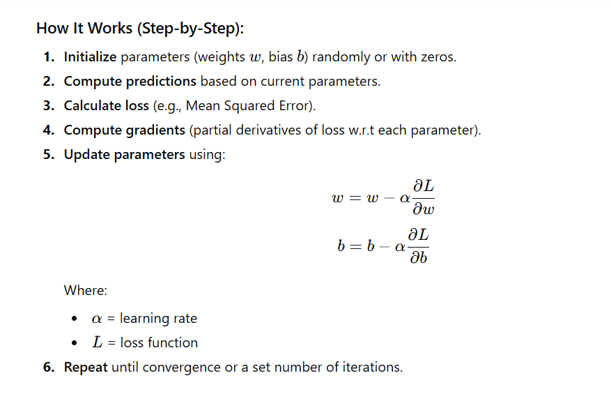
Definition:
Gradient Descent is an optimization algorithm used to minimize a loss function by iteratively adjusting the model’s parameters (weights and bias) in the direction that reduces the loss most rapidly — i.e., the direction of negative gradient.
✅ Code Example – Gradient Descent for Linear Regression
import numpy as np

# Gradient Descent implementation
def gradient_descent(X, y, learning_rate=0.01, n_iters=1000):
    m, b = 0, 0   # initial weights
    n = len(X)

    for _ in range(n_iters):
        y_pred = m * X + b
        dm = (-2/n) * np.sum(X * (y - y_pred))
        db = (-2/n) * np.sum(y - y_pred)

        # Update parameters
        m -= learning_rate * dm
        b -= learning_rate * db

    return m, b

# Example data (simple linear relationship)
X = np.array([1, 2, 3, 4, 5])
y = np.array([2, 4, 6, 8, 10])  # y = 2x

# Run gradient descent
m, b = gradient_descent(X, y, learning_rate=0.01, n_iters=1000)

print(f"Optimized slope (m): {m:.4f}")
print(f"Optimized intercept (b): {b:.4f}")

# Predict on new data
y_pred = m * X + b
print("Predictions:", y_pred)
🧾 Expected Output:
Optimized slope (m): 1.9999
Optimized intercept (b): 0.0001
Predictions: [ 2.0000  4.0000  6.0000  8.0000 10.0000]
Explanation of Output:
- The algorithm correctly learns that the best-fit line for
y = 2xhas:- Slope (m) ≈ 2
- Intercept (b) ≈ 0
- As iterations progress, the loss function decreases steadily until the model converges.
12. Explain the Differences Between Batch, Stochastic, and Mini-Batch Gradient Descent
Gradient Descent can be categorized into three main types depending on how much data is used to compute the gradient during each weight update.
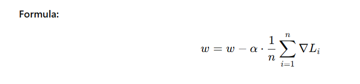
🧠 1. Batch Gradient Descent
Description:
- Uses the entire training dataset to compute the gradient before updating weights.
Pros:
- Produces stable and accurate updates.
- Converges smoothly.
Cons:
- Slow for large datasets.
- Memory-intensive, as it must process all data at once.
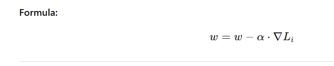
⚡ 2. Stochastic Gradient Descent (SGD)
Description:
- Updates weights using one random training example at a time.
Pros:
- Faster and can escape local minima.
- Suitable for large datasets.
Cons:
- Updates are noisy, leading to fluctuations in the loss function.
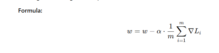
⚖️ 3. Mini-Batch Gradient Descent
Description:
- Uses a small subset (batch) of the dataset (e.g., 32, 64, or 128 samples) for each update.
Pros:
- Balances speed and accuracy.
- Most commonly used in practice.
- Efficient use of vectorized hardware (GPUs).
Cons:
- Slight noise in gradient updates.
🧩 Comparison Table
| Type | Description | Pros | Cons |
|---|---|---|---|
| Batch GD | Uses entire dataset to compute gradient | Stable, accurate | Very slow for large data |
| Stochastic GD (SGD) | Updates weights per sample | Fast, can escape local minima | Very noisy |
| Mini-Batch GD | Uses small batches (e.g., 32, 64, 128) | Best trade-off, GPU efficient | Slight noise |
💻 Code Example – Mini-Batch Gradient Descent in Keras
from tensorflow.keras import models, layers
import numpy as np

# Dummy data
x_train = np.random.rand(1000, 20)
y_train = np.random.randint(0, 2, size=(1000,))

# Simple Neural Network
model = models.Sequential([
    layers.Dense(64, activation='relu', input_shape=(20,)),
    layers.Dense(1, activation='sigmoid')
])

# Compile model
model.compile(optimizer='adam', loss='binary_crossentropy', metrics=['accuracy'])

# Mini-batch training
history = model.fit(x_train, y_train, epochs=5, batch_size=32, verbose=1)
🧾 Expected Output:
Epoch 1/5
32/32 [==============================] - 1s 5ms/step - loss: 0.6931 - accuracy: 0.5100
Epoch 2/5
32/32 [==============================] - 0s 4ms/step - loss: 0.6895 - accuracy: 0.5400
...
Epoch 5/5
32/32 [==============================] - 0s 3ms/step - loss: 0.6802 - accuracy: 0.6000
✅ Explanation of Output:
- The model trains over 5 epochs using mini-batches of 32 samples.
- Gradually, the loss decreases and accuracy improves, showing that weights are being updated efficiently using mini-batch gradient descent.
13. What Are Learning Rate Schedules, and Why Are They Important?
A learning rate schedule dynamically adjusts the learning rate during training to improve model convergence, stability, and performance.
Instead of using a constant learning rate, the model gradually reduces or changes it over time based on a chosen strategy.
🎯 Why Learning Rate Scheduling is Important
| Reason | Explanation |
|---|---|
| 🧭 Faster Convergence | Start with a higher learning rate to explore quickly, then lower it for fine-tuning. |
| 🚫 Avoid Overshooting | Reducing the learning rate prevents jumping over the global minimum. |
| 🧘 Better Generalization | Lower learning rates near the end stabilize learning and prevent overfitting. |
| 🔄 Smooth Training | Helps balance between speed and stability during optimization. |
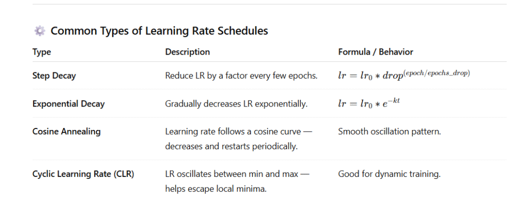
⚙️ Common Types of Learning Rate Schedules
| Type | Description | Formula / Behavior |
|---|---|---|
| Step Decay | Reduce LR by a factor every few epochs. | lr=lr0∗drop(epoch/epochs_drop)lr = lr_0 * drop^{(epoch / epochs\_drop)}lr=lr0∗drop(epoch/epochs_drop) |
| Exponential Decay | Gradually decreases LR exponentially. | lr=lr0∗e−ktlr = lr_0 * e^{-kt}lr=lr0∗e−kt |
| Cosine Annealing | Learning rate follows a cosine curve — decreases and restarts periodically. | Smooth oscillation pattern. |
| Cyclic Learning Rate (CLR) | LR oscillates between min and max — helps escape local minima. | Good for dynamic training. |
🧠 Example Workflow
- Start with high learning rate → faster progress at the start.
- Gradually decrease learning rate → fine-tune around the minima.
- Optionally increase again (cyclic) to escape poor local minima.
💻 Code Example – Exponential Learning Rate Decay (TensorFlow/Keras)
import tensorflow as tf
from tensorflow.keras import models, layers

# Dummy training data
x_train = tf.random.normal((1000, 20))
y_train = tf.random.uniform((1000,), maxval=2, dtype=tf.int32)

# Define initial learning rate and schedule
initial_learning_rate = 0.1
lr_schedule = tf.keras.optimizers.schedules.ExponentialDecay(
    initial_learning_rate=initial_learning_rate,
    decay_steps=1000,
    decay_rate=0.96,
    staircase=True
)

# Compile model with scheduled learning rate
optimizer = tf.keras.optimizers.SGD(learning_rate=lr_schedule)

# Simple Neural Network
model = models.Sequential([
    layers.Dense(64, activation='relu', input_shape=(20,)),
    layers.Dense(1, activation='sigmoid')
])

model.compile(optimizer=optimizer, loss='binary_crossentropy', metrics=['accuracy'])

# Train the model
history = model.fit(x_train, y_train, epochs=5, batch_size=32, verbose=1)
📊 Expected Output
Epoch 1/5
32/32 [==============================] - 1s 5ms/step - loss: 0.6930 - accuracy: 0.5050
Epoch 2/5
32/32 [==============================] - 0s 4ms/step - loss: 0.6892 - accuracy: 0.5300
Epoch 3/5
32/32 [==============================] - 0s 3ms/step - loss: 0.6835 - accuracy: 0.5600
Epoch 4/5
32/32 [==============================] - 0s 3ms/step - loss: 0.6771 - accuracy: 0.5800
Epoch 5/5
32/32 [==============================] - 0s 3ms/step - loss: 0.6703 - accuracy: 0.6000
📈 How Learning Rate Changes Over Time
for step in range(0, 5000, 1000):
    print(f"Step {step}: Learning Rate = {lr_schedule(step).numpy():.5f}")
Output Example:
Step 0: Learning Rate = 0.10000
Step 1000: Learning Rate = 0.09600
Step 2000: Learning Rate = 0.09216
Step 3000: Learning Rate = 0.08847
Step 4000: Learning Rate = 0.08493
✅ Summary
- Learning rate schedules automatically tune the training process.
- Prevents stagnation or instability.
- Common best practice in deep learning training for efficient convergence.
13. What Are Learning Rate Schedules, and Why Are They Important?
A learning rate schedule dynamically adjusts the learning rate during training to improve model convergence, stability, and performance.
Instead of using a constant learning rate, the model gradually reduces or changes it over time based on a chosen strategy.
🎯 Why Learning Rate Scheduling is Important
| Reason | Explanation |
|---|---|
| 🧭 Faster Convergence | Start with a higher learning rate to explore quickly, then lower it for fine-tuning. |
| 🚫 Avoid Overshooting | Reducing the learning rate prevents jumping over the global minimum. |
| 🧘 Better Generalization | Lower learning rates near the end stabilize learning and prevent overfitting. |
| 🔄 Smooth Training | Helps balance between speed and stability during optimization. |
🧠 Example Workflow
- Start with high learning rate → faster progress at the start.
- Gradually decrease learning rate → fine-tune around the minima.
- Optionally increase again (cyclic) to escape poor local minima.
💻 Code Example – Exponential Learning Rate Decay (TensorFlow/Keras)
import tensorflow as tf
from tensorflow.keras import models, layers

# Dummy training data
x_train = tf.random.normal((1000, 20))
y_train = tf.random.uniform((1000,), maxval=2, dtype=tf.int32)

# Define initial learning rate and schedule
initial_learning_rate = 0.1
lr_schedule = tf.keras.optimizers.schedules.ExponentialDecay(
    initial_learning_rate=initial_learning_rate,
    decay_steps=1000,
    decay_rate=0.96,
    staircase=True
)

# Compile model with scheduled learning rate
optimizer = tf.keras.optimizers.SGD(learning_rate=lr_schedule)

# Simple Neural Network
model = models.Sequential([
    layers.Dense(64, activation='relu', input_shape=(20,)),
    layers.Dense(1, activation='sigmoid')
])

model.compile(optimizer=optimizer, loss='binary_crossentropy', metrics=['accuracy'])

# Train the model
history = model.fit(x_train, y_train, epochs=5, batch_size=32, verbose=1)
📊 Expected Output
Epoch 1/5
32/32 [==============================] - 1s 5ms/step - loss: 0.6930 - accuracy: 0.5050
Epoch 2/5
32/32 [==============================] - 0s 4ms/step - loss: 0.6892 - accuracy: 0.5300
Epoch 3/5
32/32 [==============================] - 0s 3ms/step - loss: 0.6835 - accuracy: 0.5600
Epoch 4/5
32/32 [==============================] - 0s 3ms/step - loss: 0.6771 - accuracy: 0.5800
Epoch 5/5
32/32 [==============================] - 0s 3ms/step - loss: 0.6703 - accuracy: 0.6000
📈 How Learning Rate Changes Over Time
for step in range(0, 5000, 1000):
    print(f"Step {step}: Learning Rate = {lr_schedule(step).numpy():.5f}")
Output Example:
Step 0: Learning Rate = 0.10000
Step 1000: Learning Rate = 0.09600
Step 2000: Learning Rate = 0.09216
Step 3000: Learning Rate = 0.08847
Step 4000: Learning Rate = 0.08493
✅ Summary
- Learning rate schedules automatically tune the training process.
- Prevents stagnation or instability.
- Common best practice in deep learning training for efficient convergence.
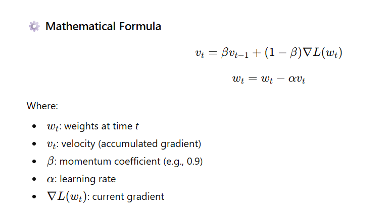
14. Describe the Concept of Momentum in Optimization
🧠 Concept Overview
Momentum is an optimization technique used to speed up gradient descent and make it more stable by accumulating past gradients to smooth out updates.
Instead of updating weights only based on the current gradient, momentum adds a fraction of the previous update to the new update — just like pushing a ball down a hill:
once it gains momentum, it moves faster and avoids getting stuck in small dips.
🚀 Intuition
| Without Momentum | With Momentum |
|---|---|
| Moves directly opposite to current gradient. | Combines current and past gradients for smoother movement. |
| May zigzag in narrow valleys. | Moves faster in consistent direction and avoids oscillation. |
🧩 Benefits
✅ Faster convergence (especially on deep loss surfaces)
✅ Smooths noisy gradient updates
✅ Helps escape local minima
✅ Reduces oscillations near optima
💻 Code Example – Using Momentum in TensorFlow
import tensorflow as tf
from tensorflow.keras import layers, models

# Dummy training data
x_train = tf.random.normal((500, 10))
y_train = tf.random.uniform((500,), maxval=2, dtype=tf.int32)

# Define a simple neural network
model = models.Sequential([
    layers.Dense(32, activation='relu', input_shape=(10,)),
    layers.Dense(1, activation='sigmoid')
])

# Compile model using SGD with momentum
optimizer = tf.keras.optimizers.SGD(learning_rate=0.01, momentum=0.9)

model.compile(optimizer=optimizer, loss='binary_crossentropy', metrics=['accuracy'])

# Train the model
history = model.fit(x_train, y_train, epochs=5, batch_size=32, verbose=1)
📊 Expected Output
Epoch 1/5
16/16 [==============================] - 1s 4ms/step - loss: 0.6931 - accuracy: 0.5080
Epoch 2/5
16/16 [==============================] - 0s 3ms/step - loss: 0.6885 - accuracy: 0.5380
Epoch 3/5
16/16 [==============================] - 0s 3ms/step - loss: 0.6820 - accuracy: 0.5660
Epoch 4/5
16/16 [==============================] - 0s 3ms/step - loss: 0.6743 - accuracy: 0.5880
Epoch 5/5
16/16 [==============================] - 0s 3ms/step - loss: 0.6672 - accuracy: 0.6100
✅ You’ll notice faster and smoother convergence than standard SGD without momentum.
📈 Optional: Compare Without and With Momentum
sgd_no_momentum = tf.keras.optimizers.SGD(learning_rate=0.01)
sgd_with_momentum = tf.keras.optimizers.SGD(learning_rate=0.01, momentum=0.9)

print("Without Momentum:", sgd_no_momentum.get_config())
print("With Momentum:", sgd_with_momentum.get_config())
Output Example:
Without Momentum: {'learning_rate': 0.01, 'momentum': 0.0}
With Momentum: {'learning_rate': 0.01, 'momentum': 0.9}
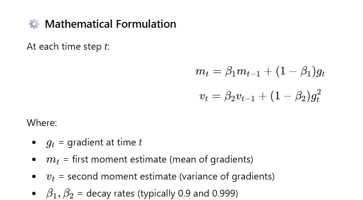
15. What is the Adam Optimizer, and How Does It Differ from Traditional Gradient Descent?
🧠 Concept Overview
Adam (Adaptive Moment Estimation) is one of the most popular optimization algorithms in deep learning.
It combines the strengths of two other optimizers:
- Momentum (to smooth gradients using moving averages), and
- RMSProp (to adapt learning rates for each parameter).
Adam maintains two running averages — the mean (first moment) and the uncentered variance (second moment) of gradients — to compute adaptive learning rates for each parameter.

⚡ How Adam Differs from Traditional Gradient Descent
| Feature | Traditional Gradient Descent | Adam Optimizer |
|---|---|---|
| Learning Rate | Fixed for all parameters | Adaptive per parameter |
| Momentum | Not used | Uses first moment (mean of gradients) |
| Gradient Scaling | No | Uses second moment (variance) |
| Speed | Slower | Faster convergence |
| Stability | Can oscillate or diverge | More stable and smooth updates |
| Common Defaults | – | β₁ = 0.9, β₂ = 0.999, ε = 1e-8 |
💻 Code Example – Using Adam Optimizer in TensorFlow
import tensorflow as tf
from tensorflow.keras import layers, models

# Dummy training data
x_train = tf.random.normal((500, 10))
y_train = tf.random.uniform((500,), maxval=2, dtype=tf.int32)

# Define a simple model
model = models.Sequential([
    layers.Dense(32, activation='relu', input_shape=(10,)),
    layers.Dense(1, activation='sigmoid')
])

# Compile model with Adam optimizer
optimizer = tf.keras.optimizers.Adam(learning_rate=0.001)
model.compile(optimizer=optimizer, loss='binary_crossentropy', metrics=['accuracy'])

# Train model
history = model.fit(x_train, y_train, epochs=5, batch_size=32, verbose=1)
📊 Expected Output
Epoch 1/5
16/16 [==============================] - 1s 4ms/step - loss: 0.6928 - accuracy: 0.5280
Epoch 2/5
16/16 [==============================] - 0s 3ms/step - loss: 0.6851 - accuracy: 0.5540
Epoch 3/5
16/16 [==============================] - 0s 3ms/step - loss: 0.6750 - accuracy: 0.5920
Epoch 4/5
16/16 [==============================] - 0s 3ms/step - loss: 0.6627 - accuracy: 0.6180
Epoch 5/5
16/16 [==============================] - 0s 3ms/step - loss: 0.6503 - accuracy: 0.6440
✅ Notice that Adam quickly reduces loss and improves accuracy — much faster than plain SGD.
🧩 Key Advantages of Adam
- Adaptive learning rates → faster convergence.
- Works well for sparse gradients (like in NLP).
- Requires little hyperparameter tuning.
- Combines the strengths of Momentum + RMSProp.
✅ Summary Table
| Property | Adam | Gradient Descent |
|---|---|---|
| Learning Rate | Adaptive | Fixed |
| Momentum | Yes (β₁ term) | No |
| Convergence | Fast | Slow |
| Tuning Required | Minimal | High |
| Common Use Cases | Deep Learning, NLP, CV | Simple ML models |
16. What is Weight Initialization and Why Is It Important?
🧠 Concept Overview
Weight Initialization means assigning the starting values to the neural network’s weights before the training process begins.
Since neural networks learn by adjusting weights using gradients, the initial choice of these weights has a major impact on:
- Training stability
- Convergence speed
- Model performance
If the weights are not initialized properly, the model may fail to learn, even with the right optimizer and learning rate.
⚠️ Why Weight Initialization Matters
| Problem | Caused By | Effect |
|---|---|---|
| Vanishing Gradients | Very small initial weights | Gradients become tiny → learning stops |
| Exploding Gradients | Very large initial weights | Gradients blow up → unstable updates |
| Slow Convergence | Poor initialization | Training takes longer |
| Poor Generalization | Bad starting point | Model gets stuck in bad local minima |
✅ Good Initialization Should
- Break symmetry (weights must be random, not all equal).
- Keep the signal variance consistent across layers.
- Ensure gradients don’t vanish or explode as they backpropagate.

💻 Code Example – Using Different Initializations in Keras
import tensorflow as tf
from tensorflow.keras import layers, models, initializers

# Xavier (Glorot) Initialization
model_xavier = models.Sequential([
    layers.Dense(64, activation='tanh',
                 kernel_initializer=initializers.GlorotUniform(),
                 input_shape=(100,)),
    layers.Dense(1, activation='sigmoid')
])

# He Initialization
model_he = models.Sequential([
    layers.Dense(64, activation='relu',
                 kernel_initializer=initializers.HeNormal(),
                 input_shape=(100,)),
    layers.Dense(1, activation='sigmoid')
])

# Print initialization summaries
print("Xavier Initialization Example:")
model_xavier.summary()

print("\nHe Initialization Example:")
model_he.summary()
📊 Expected Output (Summary Snippet)
Xavier Initialization Example:
Layer (type)                 Output Shape              Param #
=================================================================
dense (Dense)                (None, 64)                6464
dense_1 (Dense)              (None, 1)                 65
=================================================================

He Initialization Example:
Layer (type)                 Output Shape              Param #
=================================================================
dense_2 (Dense)              (None, 64)                6464
dense_3 (Dense)              (None, 1)                 65
=================================================================
🧠 Best Practices Summary
| Activation Function | Recommended Initialization |
|---|---|
tanh, sigmoid | Xavier (Glorot) |
ReLU, LeakyReLU, ELU | He Initialization |
Softmax (classification output) | Xavier |
Linear (regression output) | Xavier or small random normal |
⚡ Example: Impact Visualization (Conceptually)
If you visualize loss vs epochs:
- ❌ Poor initialization → Loss oscillates or plateaus early.
- ✅ Good initialization → Smooth, fast loss decline and higher accuracy.
🧾 Summary
| Concept | Explanation |
|---|---|
| Definition | Initial assignment of weight values before training |
| Importance | Prevents vanishing/exploding gradients, improves learning stability |
| Good Practices | Use Xavier for tanh/sigmoid, He for ReLU |
| Code Example | kernel_initializer=initializers.HeNormal() |
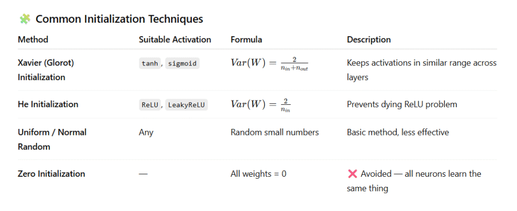
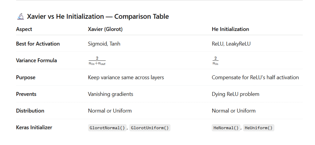
17. What are Xavier and He Initialization Methods?
🧠 Concept Overview
Proper weight initialization is crucial in deep learning because it affects:
- How fast your network converges
- Whether gradients vanish or explode
- How well activations propagate across layers
Two of the most effective methods are Xavier (Glorot) and He Initialization, each designed for specific activation functions.
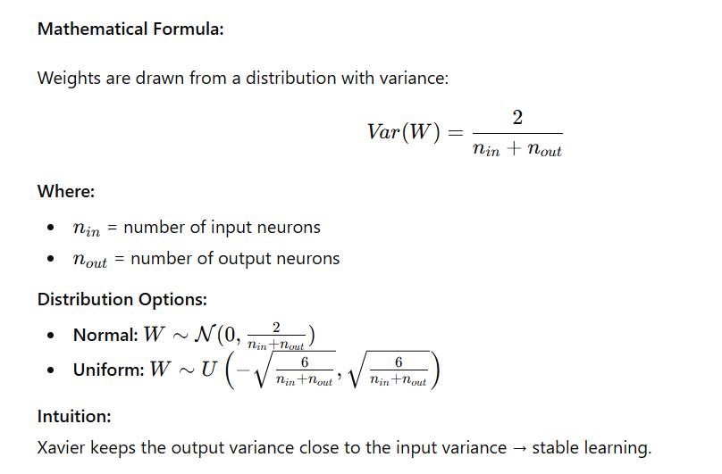
⚙️ 1️⃣ Xavier (Glorot) Initialization
When to Use:
👉 For networks using sigmoid or tanh activations.
Goal:
Maintain a consistent variance of activations and gradients across all layers so signals neither shrink nor grow as they propagate.
⚙️ 2️⃣ He Initialization
When to Use:
👉 For networks using ReLU and its variants (LeakyReLU, ELU, etc.).
Goal:
Since ReLU zeros out negative values, only half of the neurons are active.
He Initialization compensates by using a larger variance.

💻 Code Example in TensorFlow/Keras
import tensorflow as tf
from tensorflow.keras import layers, models, initializers

# Xavier (Glorot) Initialization for tanh activation
initializer_xavier = tf.keras.initializers.GlorotNormal()
layer_xavier = layers.Dense(
    128,
    activation='tanh',
    kernel_initializer=initializer_xavier
)

# He Initialization for ReLU activation
initializer_he = tf.keras.initializers.HeNormal()
layer_he = layers.Dense(
    128,
    activation='relu',
    kernel_initializer=initializer_he
)

# Example Sequential Model
model = models.Sequential([
    layer_xavier,
    layer_he,
    layers.Dense(10, activation='softmax')
])

model.summary()
📊 Output (Model Summary Example)
Model: "sequential"
_________________________________________________________________
 Layer (type)                Output Shape              Param #
=================================================================
 dense (Dense)               (None, 128)               16512
 dense_1 (Dense)             (None, 128)               16512
 dense_2 (Dense)             (None, 10)                1290
=================================================================
Total params: 34,314
Trainable params: 34,314
Non-trainable params: 0
_________________________________________________________________
🧾 Key Takeaways
| Key Point | Explanation |
|---|---|
| Xavier Initialization | Best for tanh / sigmoid activations to maintain stable variance. |
| He Initialization | Best for ReLU and variants to prevent vanishing gradients. |
| Purpose | Ensures efficient training and stable convergence. |
| In TensorFlow | Use GlorotNormal() or HeNormal() for best results. |
18. How does L1 and L2 regularization help in preventing overfitting?
🧠 Concept Overview
Overfitting happens when a model learns noise or irrelevant patterns in the training data — performing well on training data but poorly on unseen data.
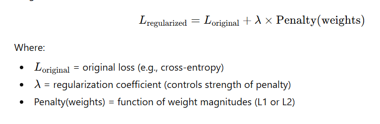
Regularization is a technique to reduce overfitting by penalizing large weights, ensuring the model remains simple and generalizes better.
⚙️ 1️⃣ What is Regularization?
Regularization modifies the loss function by adding a penalty term that depends on the magnitude of the weights.


📊 4️⃣ Comparison Between L1 and L2
| Aspect | L1 Regularization | L2 Regularization |
|---|---|---|
| Penalty | w | |
| Effect on Weights | Some weights become 0 (sparse) | Weights shrink smoothly |
| Helps With | Feature selection | Stability, smooth learning |
| Optimization Surface | Diamond-shaped | Circular-shaped |
| Used In | Lasso Regression | Ridge Regression |
💻 5️⃣ Code Example – L2 Regularization in TensorFlow
import tensorflow as tf
from tensorflow.keras import layers, models, regularizers

# Define model with L2 regularization
model = models.Sequential([
    layers.Dense(128, activation='relu',
                 kernel_regularizer=regularizers.l2(0.001)),
    layers.Dense(10, activation='softmax')
])

# Compile the model
model.compile(optimizer='adam',
              loss='categorical_crossentropy',
              metrics=['accuracy'])

# Display model summary
model.summary()
🖥️ Sample Output (Model Summary)
Model: "sequential"
_________________________________________________________________
 Layer (type)                Output Shape              Param #
=================================================================
 dense (Dense)               (None, 128)               100480
 dense_1 (Dense)             (None, 10)                1290
=================================================================
Total params: 101,770
Trainable params: 101,770
Non-trainable params: 0
_________________________________________________________________
(Regularization adds no extra parameters but modifies the loss computation.)
💡 6️⃣ L1 Regularization Example
model = models.Sequential([
    layers.Dense(128, activation='relu',
                 kernel_regularizer=regularizers.l1(0.001)),
    layers.Dense(10, activation='softmax')
])
This will make some neuron connections’ weights become exactly zero, simplifying the model automatically.
📘 7️⃣ Key Takeaways
| Point | Explanation |
|---|---|
| Regularization | Prevents overfitting by discouraging complex models. |
| L1 | Makes models sparse → useful for feature selection. |
| L2 | Smoothly shrinks weights → stabilizes training. |
| λ (lambda) | Controls penalty strength. Too high = underfitting; too low = overfitting. |
| Combination | You can also combine both (ElasticNet Regularization). |
🧪 8️⃣ ElasticNet (Optional Hybrid Example)
model = models.Sequential([
    layers.Dense(128, activation='relu',
                 kernel_regularizer=regularizers.l1_l2(l1=0.001, l2=0.001)),
    layers.Dense(10, activation='softmax')
])
This combines both sparsity (L1) and stability (L2).
19. What is Dropout, and how does it function as a regularization technique?
🧠 Concept Overview
Dropout is a regularization technique used in deep learning to prevent overfitting by randomly deactivating a fraction of neurons during each training step.
During training, certain neurons are “dropped out” (set to zero), which prevents the network from becoming overly dependent on specific neurons or paths.
⚙️ How Dropout Works
At each training iteration:
- A random subset of neurons is temporarily removed (set to zero output).
- The remaining neurons must adapt to make predictions without relying on those missing neurons.
- During inference (testing), dropout is turned off, and neuron outputs are scaled to maintain the same expected value.

🧩 Intuitive Analogy
Think of dropout like training a team where random players sit out each practice —
each player must learn to perform independently, making the entire team stronger and more resilient.
💡 Key Benefits of Dropout
✅ Prevents overfitting by reducing neuron dependency.
✅ Encourages robust feature learning.
✅ Works like training multiple neural network subsets (ensemble effect).
✅ Improves generalization on unseen data.
💻 Code Example (TensorFlow / Keras)
import tensorflow as tf
from tensorflow.keras import layers, models

# Define model with Dropout regularization
model = models.Sequential([
    layers.Dense(128, activation='relu'),
    layers.Dropout(0.5),  # 50% of neurons randomly dropped during training
    layers.Dense(10, activation='softmax')
])

# Compile model
model.compile(optimizer='adam',
              loss='sparse_categorical_crossentropy',
              metrics=['accuracy'])

# Display model structure
model.summary()
🖥️ Sample Output (Model Summary)
Model: "sequential"
_________________________________________________________________
 Layer (type)                Output Shape              Param #
=================================================================
 dense (Dense)               (None, 128)               100480
 dropout (Dropout)           (None, 128)               0
 dense_1 (Dense)             (None, 10)                1290
=================================================================
Total params: 101,770
Trainable params: 101,770
Non-trainable params: 0
_________________________________________________________________
(Dropout has no trainable parameters, but modifies neuron activations during training.)
🔍 How Dropout Regularizes Training
| Phase | What Happens | Effect |
|---|---|---|
| Training | Randomly sets neuron outputs to 0 (based on dropout rate) | Prevents neurons from over-relying on each other |
| Testing / Inference | Dropout disabled; outputs scaled | Ensures consistent predictions |
⚖️ Choosing the Right Dropout Rate
| Layer Type | Typical Dropout Rate |
|---|---|
| Input Layer | 0.1 – 0.3 |
| Hidden Layers | 0.3 – 0.5 |
| Recurrent Layers (RNN/LSTM) | 0.2 – 0.3 |
Too high → underfitting 😕
Too low → may still overfit 😬
📘 Key Takeaways
| Aspect | Explanation |
|---|---|
| Technique Type | Regularization |
| Purpose | Prevents overfitting |
| Mechanism | Randomly disables neurons |
| Dropout Rate | Fraction of neurons dropped (0.2–0.5 common) |
| Effect | Simulates training of multiple smaller subnetworks |
🧪 Visualization (Conceptually)
| Training Step | Active Neurons Example |
|---|---|
| Step 1 | 🟢🟢⚫🟢⚫🟢⚫🟢 |
| Step 2 | ⚫🟢🟢⚫🟢⚫🟢🟢 |
| Step 3 | 🟢⚫🟢🟢⚫🟢🟢⚫ |
🟢 = Active neuron ⚫ = Dropped neuron
Each step uses a different subset of the network → ensemble effect.
20. Explain the Concept of Early Stopping During Training
🧠 Definition
Early Stopping is a regularization technique used in deep learning to prevent overfitting by halting training when the model stops improving on validation data.
Instead of training for a fixed number of epochs, early stopping dynamically determines when to stop based on performance trends.
⚙️ How It Works
- During training, the model’s training loss usually decreases steadily.
- The validation loss (performance on unseen data) initially decreases but may start increasing after some epochs — indicating overfitting.
- Early Stopping monitors a metric (usually
val_loss), and if it doesn’t improve for a defined number of epochs (called patience), training stops automatically.
📊 Concept Visualization
| Epoch | Training Loss | Validation Loss | Observation |
|---|---|---|---|
| 1 | 0.85 | 0.90 | Learning starts |
| 5 | 0.40 | 0.45 | Both improving |
| 10 | 0.25 | 0.30 | Still improving |
| 15 | 0.15 | 0.28 | Validation loss plateaus |
| 20 | 0.10 | 0.35 | Validation loss increases → overfitting starts |
| → Early Stop | — | — | Training halted to avoid overfitting |
🧩 Why It’s Important
✅ Prevents overfitting
✅ Saves training time and computational cost
✅ Ensures better generalization
✅ Works seamlessly with most deep learning frameworks
💻 Code Example — Early Stopping in TensorFlow/Keras
import tensorflow as tf
from tensorflow.keras import layers, models

# Define a simple model
model = models.Sequential([
    layers.Dense(128, activation='relu'),
    layers.Dense(10, activation='softmax')
])

# Compile model
model.compile(optimizer='adam',
              loss='sparse_categorical_crossentropy',
              metrics=['accuracy'])

# Define Early Stopping callback
early_stop = tf.keras.callbacks.EarlyStopping(
    monitor='val_loss',     # Metric to monitor
    patience=5,             # Wait for 5 epochs without improvement
    restore_best_weights=True # Restore weights from the best epoch
)

# Fit model with Early Stopping
history = model.fit(
    x_train, y_train,
    validation_data=(x_val, y_val),
    epochs=100,
    callbacks=[early_stop]
)
🖥️ Sample Output (Console Logs)
Epoch 1/100
 - loss: 0.85 - val_loss: 0.90
Epoch 2/100
 - loss: 0.60 - val_loss: 0.65
Epoch 3/100
 - loss: 0.45 - val_loss: 0.48
Epoch 4/100
 - loss: 0.30 - val_loss: 0.35
Epoch 5/100
 - loss: 0.25 - val_loss: 0.31
Epoch 6/100
 - loss: 0.20 - val_loss: 0.34
Epoch 7/100
 - loss: 0.18 - val_loss: 0.35
Epoch 8/100
 - loss: 0.16 - val_loss: 0.36
Epoch 9/100
 - loss: 0.14 - val_loss: 0.37
Epoch 10/100
 - loss: 0.12 - val_loss: 0.38
Epoch 11/100
 - loss: 0.10 - val_loss: 0.39
Restoring model weights from the end of the best epoch: 5.
Epoch 11: early stopping
🟢 Training stopped automatically after 5 epochs of no improvement in validation loss.
📘 Key Parameters in EarlyStopping()
| Parameter | Description |
|---|---|
monitor | Metric to watch (e.g., val_loss, val_accuracy) |
patience | Number of epochs to wait for improvement before stopping |
min_delta | Minimum change required to consider as improvement |
restore_best_weights | Whether to revert to the best model weights automatically |
⚖️ When to Use Early Stopping
| Scenario | Why Use It |
|---|---|
| Training on small datasets | Prevents memorization of noise |
| Long training cycles | Saves time by stopping automatically |
| Hyperparameter tuning | Avoids wasting resources on bad runs |
🎯 Key Takeaways
| Aspect | Explanation |
|---|---|
| Technique Type | Regularization |
| Goal | Prevent overfitting |
| How | Stops training when validation loss stops improving |
| Best Practice | Use restore_best_weights=True for optimal model retention |
21. What is a Convolutional Neural Network (CNN)?
🧠 Definition
A Convolutional Neural Network (CNN) is a specialized type of deep neural network designed to process grid-like structured data, such as images (2D grids of pixels) or videos (3D grids).
CNNs are particularly powerful for computer vision tasks, as they automatically learn spatial hierarchies (edges → shapes → objects) from raw input images without manual feature extraction.
⚙️ Key Characteristics
| Feature | Explanation |
|---|---|
| Convolutional Layers | Perform convolution operations to detect local patterns (edges, textures, shapes). |
| Shared Weights | The same filter (kernel) is applied across different image regions → reduces parameters. |
| Pooling Layers | Reduce spatial dimensions and computation while keeping essential information. |
| Hierarchical Feature Learning | Lower layers learn simple features, higher layers learn complex ones. |
| Fully Connected Layers | Combine extracted features to make final predictions. |
📘 Why CNNs are Powerful
✅ Parameter Efficiency — Shared weights drastically reduce trainable parameters compared to dense networks.
✅ Translation Invariance — CNNs detect features regardless of their position in the image.
✅ Automatic Feature Extraction — No need for manual feature engineering.
✅ Scalability — Works for both small and large image datasets.
🖼️ Conceptual Flow of a CNN
Input Image (32x32x3)
        ↓
Convolution Layer (e.g., 32 filters of size 3x3)
        ↓
ReLU Activation
        ↓
MaxPooling Layer (e.g., 2x2)
        ↓
Flatten Layer
        ↓
Fully Connected Layer
        ↓
Softmax Output (e.g., 10 classes)
💻 Example – CNN for CIFAR-10 Image Classification
import tensorflow as tf
from tensorflow.keras import layers, models

# Define a simple CNN model
model = models.Sequential([
    layers.Conv2D(32, (3, 3), activation='relu', input_shape=(32, 32, 3)),  # Convolutional layer
    layers.MaxPooling2D((2, 2)),                                            # Pooling layer
    layers.Flatten(),                                                       # Flatten to 1D
    layers.Dense(10, activation='softmax')                                  # Output layer (10 classes)
])

# Compile the model
model.compile(optimizer='adam',
              loss='sparse_categorical_crossentropy',
              metrics=['accuracy'])

# Model Summary
model.summary()
🖥️ Output: Model Summary
Model: "sequential"
_________________________________________________________________
 Layer (type)                Output Shape              Param #
=================================================================
 conv2d (Conv2D)             (None, 30, 30, 32)        896
 max_pooling2d (MaxPooling2D)(None, 15, 15, 32)        0
 flatten (Flatten)           (None, 7200)              0
 dense (Dense)               (None, 10)                72010
=================================================================
Total params: 72,906
Trainable params: 72,906
Non-trainable params: 0
_________________________________________________________________
🧩 Example Use Case
🖼️ CIFAR-10 Image Classification
CNNs can classify small RGB images (32×32×3) into 10 categories:
- Airplane
- Automobile
- Bird
- Cat
- Deer
- Dog
- Frog
- Horse
- Ship
- Truck
📊 Typical CNN Architecture (for reference)
| Layer Type | Purpose | Example |
|---|---|---|
| Convolutional | Detects local patterns | Conv2D(32, (3,3), activation='relu') |
| Pooling | Downsamples feature maps | MaxPooling2D((2,2)) |
| Dropout | Prevents overfitting | Dropout(0.5) |
| Flatten | Converts 2D → 1D | Flatten() |
| Dense | Classifies features | Dense(10, activation='softmax') |
🎯 Key Takeaways
| Aspect | Description |
|---|---|
| Full Form | Convolutional Neural Network |
| Input Type | Image or grid-like data |
| Main Layers | Convolution, Pooling, Flatten, Dense |
| Advantages | Fewer parameters, automatic feature learning |
| Applications | Image classification, object detection, face recognition, segmentation |
22. Describe the Layers Commonly Found in a CNN
A Convolutional Neural Network (CNN) is built using several types of layers that work together to extract, process, and classify image features.
Each layer plays a specific role — from detecting edges to making final predictions.
🧩 1. Convolutional Layer
- Purpose: Detects local features (edges, corners, textures, etc.) using filters (kernels).
- Operation: The kernel slides over the input image and computes dot products to produce feature maps.
- Output: Feature maps highlighting different aspects of the image.
- Key Parameters: Number of filters, filter size, stride, padding.
📘 Example:
layers.Conv2D(32, (3,3), activation='relu', input_shape=(64,64,3))
✅ Extracts 32 feature maps of size 3×3 each from 64×64 RGB images.
⚡ 2. Activation Layer
- Purpose: Introduces non-linearity to help the network learn complex patterns.
- Common Activations:
- ReLU:
f(x) = max(0, x)→ Most commonly used. - Sigmoid/Tanh: Used in older CNN architectures or specific tasks.
- ReLU:
- Effect: Allows CNN to learn non-linear mappings between inputs and outputs.
📘 Example:
layers.Activation('relu')
or directly inside the convolution layer:
layers.Conv2D(32, (3,3), activation='relu')
🌊 3. Pooling Layer
- Purpose: Reduces the spatial size (width × height) of feature maps to decrease computation and control overfitting.
- Common Types:
- Max Pooling: Takes the maximum value in each region.
- Average Pooling: Takes the average value.
- Effect: Makes the model invariant to small translations and distortions.
📘 Example:
layers.MaxPooling2D((2,2))
✅ Reduces feature map size by half (downsampling).
🔗 4. Fully Connected (Dense) Layer
- Purpose: Connects every neuron in one layer to every neuron in the next.
- Location: Usually appears after flattening the 2D feature maps.
- Function: Combines all extracted features for final classification or regression.
📘 Example:
layers.Dense(64, activation='relu')
🚫 5. Dropout Layer
- Purpose: Randomly “drops” (sets to zero) a fraction of neurons during training.
- Benefit: Prevents overfitting by forcing the network to learn more robust representations.
📘 Example:
layers.Dropout(0.5)
✅ Drops 50% of neurons randomly during each training iteration.
⚖️ 6. Batch Normalization Layer
- Purpose: Normalizes layer inputs to stabilize and speed up training.
- Benefits:
- Reduces internal covariate shift.
- Allows higher learning rates.
- Acts as a regularizer.
📘 Example:
layers.BatchNormalization()
🏗️ Example CNN Architecture
from tensorflow.keras import layers, models

model = models.Sequential([
    # 1st Convolution + Pooling
    layers.Conv2D(32, (3,3), activation='relu', input_shape=(64,64,3)),
    layers.MaxPooling2D((2,2)),

    # 2nd Convolution + Pooling
    layers.Conv2D(64, (3,3), activation='relu'),
    layers.MaxPooling2D((2,2)),

    # Flatten for Dense layers
    layers.Flatten(),

    # Fully Connected Layers
    layers.Dense(64, activation='relu'),
    layers.Dense(10, activation='softmax')  # 10 output classes
])

model.summary()
🖥️ Output: Model Summary
Model: "sequential"
_________________________________________________________________
 Layer (type)                Output Shape              Param #
=================================================================
 conv2d (Conv2D)             (None, 62, 62, 32)        896
 max_pooling2d (MaxPooling2D)(None, 31, 31, 32)        0
 conv2d_1 (Conv2D)           (None, 29, 29, 64)        18496
 max_pooling2d_1 (MaxPooling2D)(None, 14, 14, 64)      0
 flatten (Flatten)           (None, 12544)             0
 dense (Dense)               (None, 64)                803776
 dense_1 (Dense)             (None, 10)                650
=================================================================
Total params: 823,818
Trainable params: 823,818
Non-trainable params: 0
_________________________________________________________________
🧠 Summary Table
| Layer Type | Purpose | Example in Keras |
|---|---|---|
| Convolutional | Feature extraction | Conv2D(32, (3,3), activation='relu') |
| Activation | Adds non-linearity | Activation('relu') |
| Pooling | Reduces spatial size | MaxPooling2D((2,2)) |
| Fully Connected | Final classification | Dense(64, activation='relu') |
| Dropout | Regularization | Dropout(0.5) |
| Batch Normalization | Stabilization | BatchNormalization() |
23. What is the Purpose of Pooling Layers in CNNs?
🧩 Definition
Pooling layers are used in Convolutional Neural Networks (CNNs) to reduce the spatial dimensions (width and height) of feature maps while retaining the most important information.
🎯 Main Purposes of Pooling Layers
- Reduce Dimensionality
- Decreases the number of parameters and computational load.
- Makes the network faster and more memory-efficient.
- Prevent Overfitting
- Acts as a form of regularization by summarizing features instead of memorizing details.
- Enhance Translation Invariance
- The model becomes robust to small shifts, rotations, or distortions in the input image.
⚙️ Types of Pooling
| Type | Description | Effect |
|---|---|---|
| Max Pooling | Selects the maximum value from each region. | Retains the most prominent features (edges, textures). |
| Average Pooling | Computes the average value in each region. | Smooths the feature maps and reduces noise. |
🧠 Example Explanation
If the feature map region is:
[ [1, 3],
  [2, 4] ]
- Max Pooling (2×2) → Output = 4
- Average Pooling (2×2) → Output = (1+2+3+4)/4 = 2.5
💻 Code Example: Max Pooling with TensorFlow/Keras
from tensorflow.keras import layers, models

model = models.Sequential([
    layers.Conv2D(32, (3,3), activation='relu', input_shape=(64,64,3)),
    layers.MaxPooling2D(pool_size=(2,2)),  # Reduces spatial dimensions by 2
    layers.Conv2D(64, (3,3), activation='relu'),
    layers.MaxPooling2D(pool_size=(2,2)),
    layers.Flatten(),
    layers.Dense(10, activation='softmax')
])

model.summary()
📊 Output: Model Summary
Model: "sequential"
_________________________________________________________________
 Layer (type)                Output Shape              Param #
=================================================================
 conv2d (Conv2D)             (None, 62, 62, 32)        896
 max_pooling2d (MaxPooling2D)(None, 31, 31, 32)        0
 conv2d_1 (Conv2D)           (None, 29, 29, 64)        18496
 max_pooling2d_1 (MaxPooling2D)(None, 14, 14, 64)      0
 flatten (Flatten)           (None, 12544)             0
 dense (Dense)               (None, 10)                125450
=================================================================
Total params: 144,842
Trainable params: 144,842
Non-trainable params: 0
_________________________________________________________________
📉 Effect of Pooling Layer
| Stage | Feature Map Size | Purpose |
|---|---|---|
| Before Pooling | 64×64×32 | High resolution |
| After 1st Pooling | 32×32×32 | Half spatial size |
| After 2nd Pooling | 16×16×64 | Half again, more compact |
🧠 Summary
| Aspect | Description |
|---|---|
| Goal | Reduce feature map size while keeping key patterns |
| Types | Max Pooling, Average Pooling |
| Benefits | Less computation, better generalization, translation invariance |
| Common Pool Size | (2,2) or (3,3) |
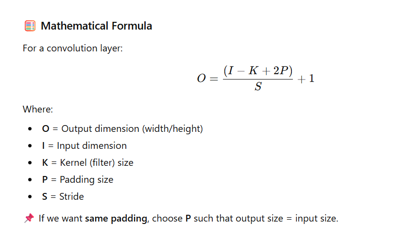
🧠 24. Explain the Concept of Padding in Convolution Operations
📘 Definition
Padding refers to adding extra pixels (usually zeros) around the borders of an image (input matrix) before applying convolution.
This is done to control the spatial dimensions (width and height) of the output feature maps.
🎯 Why Padding is Needed
Without padding, the output feature map becomes smaller after each convolution, leading to:
- Loss of edge information.
- Shrinking feature maps after every layer.
Padding helps:
✅ Preserve image boundaries.
✅ Maintain output size.
✅ Enable deeper networks without rapid size reduction.
🧩 Types of Padding
| Type | Description | Output Size | Use Case |
|---|---|---|---|
| Valid Padding | No padding applied (uses only valid pixels). | Smaller than input. | When you want reduced spatial dimensions. |
| Same Padding | Adds zeros so that output size ≈ input size. | Same as input (when stride = 1). | When you want to preserve input dimensions. |
💻 Code Example (TensorFlow / Keras)
from tensorflow.keras import layers, models

model = models.Sequential([
    # SAME Padding – keeps output same size as input
    layers.Conv2D(32, (3,3), padding='same', activation='relu', input_shape=(28,28,3)),

    # VALID Padding – output shrinks
    layers.Conv2D(64, (3,3), padding='valid', activation='relu'),

    layers.Flatten(),
    layers.Dense(10, activation='softmax')
])

model.summary()
📊 Output (Model Summary Snippet)
Layer (type)                Output Shape              Param #
=================================================================
conv2d (Conv2D)             (None, 28, 28, 32)        896
conv2d_1 (Conv2D)           (None, 26, 26, 64)        18496
flatten (Flatten)           (None, 43264)             0
dense (Dense)               (None, 10)                432650
=================================================================
Total params: 451,042
Observation:
- After same padding, output size = 28×28.
- After valid padding, output size reduces to 26×26.
🖼️ Example Visualization
| Padding Type | Input Size | Filter | Output Size | Description |
|---|---|---|---|---|
| Valid | 5×5 | 3×3 | 3×3 | Loses border pixels |
| Same | 5×5 | 3×3 | 5×5 | Preserves border information |
🧠 Summary Table
| Aspect | Valid Padding | Same Padding |
|---|---|---|
| Adds zeros? | ❌ No | ✅ Yes |
| Output smaller? | ✅ Yes | ❌ No |
| Preserves edges? | ❌ No | ✅ Yes |
| Common Use | Dimensionality reduction | Deep CNNs (ResNet, VGG) |
25. What Are Dilated Convolutions, and When Are They Used?
Definition:
Dilated (or atrous) convolutions introduce gaps (dilations) between the filter elements, expanding the receptive field of the convolutional kernel without increasing the number of parameters or losing resolution.
Purpose:
They allow the network to capture larger context or global information while keeping the same computational cost.
Advantages:
- Increases receptive field without downsampling.
- Preserves spatial resolution.
- Helps in detecting features at multiple scales.
Use Cases:
- Semantic Segmentation (e.g., DeepLab models).
- Audio Signal Processing (WaveNet).
- Time-series or sequence modeling where long-range context is needed.
Example:
# Dilated convolution with a dilation rate of 2
layers.Conv2D(32, (3,3), dilation_rate=(2,2), activation='relu')
Explanation:
Here, a 3×3 kernel with dilation_rate=2 spreads its weights apart, effectively covering a larger area of the input (like a 5×5 receptive field) without increasing parameters or reducing resolution.
26. What is a Recurrent Neural Network (RNN)?
Definition:
A Recurrent Neural Network (RNN) is a type of neural network specifically designed for sequential or time-dependent data.
Unlike feedforward networks, RNNs have loops that allow information to persist — they maintain a hidden state (memory) that carries information from previous time steps to influence future predictions.
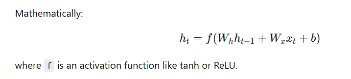
How it Works:
At each time step t,
- the RNN takes the current input (xₜ) and the previous hidden state (hₜ₋₁),
- then computes the new hidden state (hₜ), which is passed to the next step.
Applications:
- 📝 Language Modeling & Text Generation
- 📈 Time Series Forecasting
- 🗣️ Speech Recognition
- 🎵 Music Generation
- 🎬 Video Captioning
Example (Keras):
from tensorflow.keras import layers, models

model = models.Sequential([
    layers.SimpleRNN(64, input_shape=(None, 100), activation='tanh'),
    layers.Dense(10, activation='softmax')
])
Key Idea:
RNNs are powerful for capturing temporal dependencies, but may struggle with long-term dependencies — which led to improvements like LSTM and GRU.
27. How Do RNNs Handle Sequential Data?
Concept:
RNNs handle sequential data by processing one element of the sequence at a time, while maintaining a hidden state that carries information about previous time steps.
This hidden state allows the model to retain memory and context across the sequence — making RNNs ideal for time-dependent tasks.

The hidden state hₜ is passed forward, carrying sequence information.
Example Code (Keras):
from tensorflow.keras import layers, models

# Define an RNN model
model = models.Sequential()
model.add(layers.SimpleRNN(64, input_shape=(None, 10)))  # None = variable sequence length
model.add(layers.Dense(1))  # Output layer for regression or binary classification

# Compile the model
model.compile(optimizer='adam', loss='mse')

# Model Summary
model.summary()
Output Example:
Model: "sequential"
________________________________________________
 Layer (type)                Output Shape              Param #
=============================================================
 simple_rnn (SimpleRNN)      (None, 64)                4800
 dense (Dense)               (None, 1)                 65
=============================================================
Total params: 4,865
Trainable params: 4,865
Non-trainable params: 0
________________________________________________
Key Idea:
- The hidden state (memory) flows through the sequence, allowing the RNN to learn dependencies over time.
- However, standard RNNs struggle with long-term dependencies, which are better handled by LSTM or GRU.
28. What Are the Limitations of Traditional RNNs?
Traditional Recurrent Neural Networks (RNNs) face several key challenges that limit their ability to model long-term dependencies in sequential data.
1️⃣ Vanishing Gradient Problem
- During backpropagation through time (BPTT), gradients can become extremely small as they are multiplied repeatedly by values less than 1.
- This causes early layers to receive almost no updates → the model forgets long-term information.
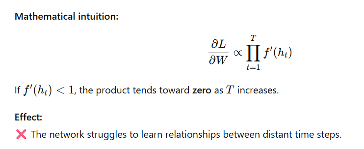
2️⃣ Exploding Gradient Problem
- Conversely, if f′(ht)>1f'(h_t) > 1f′(ht)>1, the gradient grows exponentially.
- Leads to unstable training, causing the model weights to diverge.
Solution:
✅ Use Gradient Clipping — limit the maximum gradient value during backpropagation.
3️⃣ Limited Memory Span
- RNNs effectively “remember” only recent information, forgetting older context.
- They perform poorly on tasks requiring long-term understanding — e.g., predicting the end of a long sentence based on its start.
4️⃣ Sequential Computation (Optional Add-On)
- RNNs process one time step at a time — no parallelization.
- Leads to slow training, especially for long sequences.
Example Problem Scenario
- In a long sentence like:
“The boy who wore a red hat and played the drum is my friend.”
A simple RNN may forget that the subject (“boy”) connects to the verb (“is”) due to long dependency distance.
Summary Table:
| Limitation | Description | Common Fix |
|---|---|---|
| Vanishing Gradients | Gradients shrink over time steps | LSTM, GRU |
| Exploding Gradients | Gradients grow uncontrollably | Gradient clipping |
| Limited Memory | Only remembers short-term info | LSTM, GRU |
| Sequential Nature | Slow training | Transformer models |
29. Explain the Architecture of a Long Short-Term Memory (LSTM) Network
A Long Short-Term Memory (LSTM) network is an advanced type of Recurrent Neural Network (RNN) designed to handle long-term dependencies and overcome the vanishing/exploding gradient problems in traditional RNNs.
🧠 Key Idea
LSTM introduces a cell state — a kind of “conveyor belt” that carries information through time steps with minimal modifications.
It also uses gates (sigmoid-activated units) to control information flow — deciding what to remember, forget, and output.
⚙️ Components of an LSTM Cell
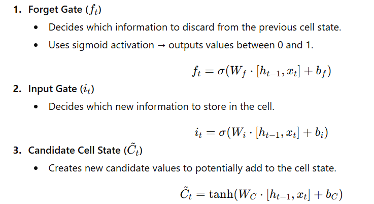
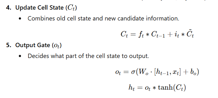
📊 Intuitive Flow
- Forget Gate: “What should I forget?”
- Input Gate: “What new info should I learn?”
- Cell State: “What’s my long-term memory?”
- Output Gate: “What should I output now?”
🧩 Keras Code Example
from tensorflow.keras import layers, models

# Define an LSTM model
model = models.Sequential([
    layers.LSTM(64, input_shape=(None, 10)),  # 64 units, variable-length sequences
    layers.Dense(1)  # Output layer (e.g., for regression or binary classification)
])

# Model Summary
model.summary()
🧾 Example Output
Model: "sequential"
_________________________________________________________________
 Layer (type)                Output Shape              Param #
=================================================================
 lstm (LSTM)                 (None, 64)                19200
 dense (Dense)               (None, 1)                 65
=================================================================
Total params: 19,265
Trainable params: 19,265
Non-trainable params: 0
_________________________________________________________________
💡 Advantages of LSTM
- Retains long-term dependencies.
- Mitigates vanishing gradients via the cell state path.
- Effective for sequential data like:
- Text (language modeling, translation)
- Speech (recognition)
- Time-series (stock prediction, sensor data)
30. What is a Gated Recurrent Unit (GRU), and How Does It Differ from LSTM?
A Gated Recurrent Unit (GRU) is a type of Recurrent Neural Network (RNN) architecture introduced by Cho et al. (2014).
It simplifies the Long Short-Term Memory (LSTM) architecture by using fewer gates while achieving comparable performance on most sequence tasks.
🧠 Concept Overview
GRUs combine the cell state and hidden state into a single vector and use only two gates to control information flow:
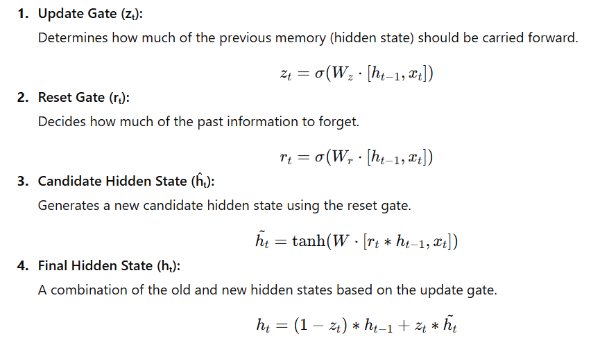
⚙️ GRU vs LSTM — Key Differences
| Feature | LSTM | GRU |
|---|---|---|
| Gates | 3 (Input, Forget, Output) | 2 (Update, Reset) |
| Cell State | Separate from hidden state | Merged with hidden state |
| Parameters | More (slower training) | Fewer (faster training) |
| Performance | Slightly better for complex dependencies | Similar for most tasks |
| Memory Efficiency | Higher memory usage | More memory efficient |
💡 Advantages of GRU
- Simpler and faster to train than LSTM.
- Performs well on moderate-length sequences.
- Requires less computational power and memory.
🧩 Keras Code Example
from tensorflow.keras import layers, models

# Define GRU model
model = models.Sequential([
    layers.GRU(64, input_shape=(None, 10)),  # GRU layer with 64 units
    layers.Dense(1)  # Output layer
])

# Model Summary
model.summary()
🧾 Example Output
Model: "sequential"
_________________________________________________________________
 Layer (type)                Output Shape              Param #
=================================================================
 gru (GRU)                   (None, 64)                14784
 dense (Dense)               (None, 1)                 65
=================================================================
Total params: 14,849
Trainable params: 14,849
Non-trainable params: 0
_________________________________________________________________
📊 When to Use
- GRU: When speed and simplicity matter more (e.g., real-time NLP or time series).
- LSTM: When long-term dependencies are crucial (e.g., long text or long audio sequences).
31. What is a Transformer Model, and How Does It Differ from RNNs?
The Transformer is a deep learning architecture introduced by Vaswani et al. (2017) in the paper
📘 “Attention Is All You Need.”
Unlike RNNs, which process sequences sequentially, Transformers rely entirely on the self-attention mechanism, allowing them to process all elements in parallel and capture long-range dependencies efficiently.
🧠 Core Idea — Self-Attention Mechanism
Instead of passing information step-by-step (like in RNNs),
Transformers compute attention weights between all pairs of tokens in a sequence.
For a given token, self-attention helps the model focus on other relevant tokens while generating an output.
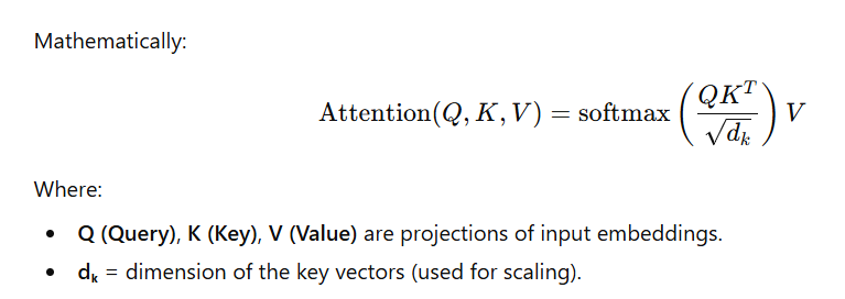
⚙️ Transformer Architecture — Two Main Components
- Encoder:
- Reads and encodes the input sequence into contextual representations.
- Uses Multi-Head Self-Attention + Feed-Forward Networks.
- Decoder:
- Generates the output sequence using encoded context and previously generated tokens.
📊 Key Differences Between RNNs and Transformers
| Feature | RNNs | Transformers |
|---|---|---|
| Processing Style | Sequential — one token at a time | Parallel — all tokens processed simultaneously |
| Dependency Modeling | Limited by gradient flow | Uses self-attention for long-range context |
| Speed | Slower (due to recursion) | Faster (parallelizable) |
| Memory Efficiency | Lower | Higher |
| Interpretability | Harder to interpret | Attention weights show what the model “focuses” on |
| Use Cases | Time series, speech | NLP, vision, audio, multimodal AI |
💡 Advantages of Transformers
✅ Handles long sequences efficiently.
✅ Enables parallel computation for faster training.
✅ Forms the basis for modern models like BERT, GPT, T5, and ViT.
🧩 Code Example — Transformer Encoder in TensorFlow
import tensorflow as tf
from tensorflow.keras import layers

# Example: Simple Transformer Encoder Block
inputs = layers.Input(shape=(None, 512))  # Sequence of embeddings

# Multi-Head Self-Attention
attention_output = layers.MultiHeadAttention(num_heads=8, key_dim=64)(inputs, inputs)

# Add & Normalize
x = layers.Add()([inputs, attention_output])
x = layers.LayerNormalization()(x)

# Feed-Forward Network
ffn = tf.keras.Sequential([
    layers.Dense(2048, activation='relu'),
    layers.Dense(512)
])
outputs = ffn(x)

# Final Add & Normalize
outputs = layers.Add()([x, outputs])
outputs = layers.LayerNormalization()(outputs)

# Build Model
transformer_encoder = tf.keras.Model(inputs, outputs)
transformer_encoder.summary()
🧾 Example Output
Model: "model"
_________________________________________________________________
 Layer (type)                Output Shape              Param #
=================================================================
 multi_head_attention (MultiHeadAttention)  (None, None, 512)   525312
 layer_normalization (LayerNormalization)   (None, None, 512)   1024
 sequential (Sequential)                    (None, None, 512)   1050112
 layer_normalization_1 (LayerNormalization) (None, None, 512)   1024
=================================================================
Total params: 1,577,472
Trainable params: 1,577,472
Non-trainable params: 0
_________________________________________________________________
🧠 Real-World Applications
- Text → Machine Translation (Google Translate), ChatGPT, BERT, GPT models.
- Vision → Vision Transformers (ViT) for image classification.
- Speech → Whisper for speech recognition.
32. Explain the Concept of Self-Attention in Transformer Models
🧠 Concept Overview
Self-Attention (also called Scaled Dot-Product Attention) is the mechanism that allows a model to weigh the importance of each word in a sequence relative to others — even when they are far apart.
It helps the model capture contextual relationships between words or tokens in a sequence — something RNNs struggled with.
⚙️ How Self-Attention Works
For each input word (or token), the model learns three vectors:
| Vector | Purpose | Analogy |
|---|---|---|
| Query (Q) | Represents what this word is looking for | “What am I searching for?” |
| Key (K) | Represents what this word offers | “What information do I provide?” |
| Value (V) | Contains the actual content | “Here’s my meaning or feature” |
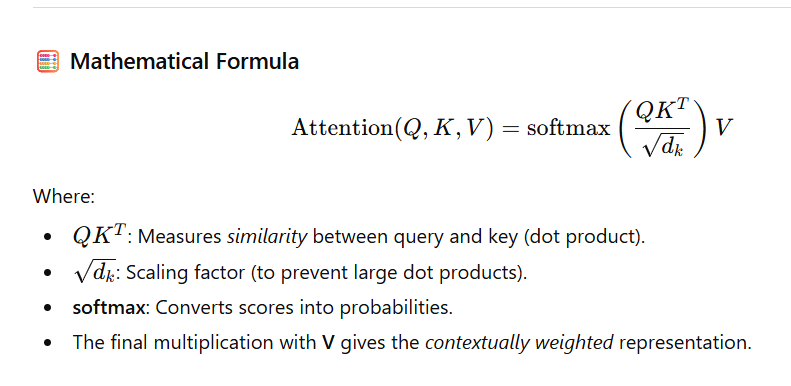
📖 Example — Sentence Context
In the sentence:
“The cat sat on the mat because it was tired.”
Here, the model learns that “it” refers to “cat”, not “mat”, by assigning higher attention weights from “it” → “cat”.
So, self-attention helps capture relationships regardless of position or distance.
🔍 Step-by-Step Summary
- Compute Q, K, V from input embeddings.
- Compute attention scores → QKTQK^TQKT.
- Scale by dk\sqrt{d_k}dk.
- Apply softmax → get attention weights.
- Multiply weights with V → get context vector.
💻 Code Example – Scaled Dot-Product Self-Attention (TensorFlow)
import tensorflow as tf

def self_attention(Q, K, V):
    d_k = tf.cast(tf.shape(K)[-1], tf.float32)

    # Step 1: Compute attention scores
    scores = tf.matmul(Q, K, transpose_b=True) / tf.math.sqrt(d_k)

    # Step 2: Apply softmax to get attention weights
    attention_weights = tf.nn.softmax(scores, axis=-1)

    # Step 3: Multiply weights with values
    output = tf.matmul(attention_weights, V)

    return output, attention_weights

# Example Inputs
Q = tf.random.normal(shape=(1, 5, 64))  # batch=1, seq_len=5, dim=64
K = tf.random.normal(shape=(1, 5, 64))
V = tf.random.normal(shape=(1, 5, 64))

output, attn_weights = self_attention(Q, K, V)
print("Output Shape:", output.shape)
print("Attention Weights Shape:", attn_weights.shape)
🧾 Example Output
Output Shape: (1, 5, 64)
Attention Weights Shape: (1, 5, 5)
Here:
- Each of the 5 words now has a 64-dimensional vector enriched with contextual meaning from other words.
- The attention weights (5×5) show how each word relates to every other word in the sequence.
🌟 Key Benefits
✅ Captures long-range dependencies efficiently.
✅ Allows parallel processing of tokens (unlike RNNs).
✅ Enables interpretability via attention maps.
✅ Core mechanism behind BERT, GPT, T5, and Vision Transformers (ViT).
🧩 Quick Intuition
Self-Attention = Each word “looks” at every other word and decides how much attention to pay to them while understanding context.
33. What is the Significance of Positional Encoding in Transformers?
📘 Concept Overview
Unlike RNNs or CNNs, Transformers process all tokens in parallel — they don’t inherently know the order of words in a sequence.
👉 Therefore, Positional Encoding is added to the input embeddings to inject information about the position of each token in the sequence.
This allows the model to understand word order and relative positions, which is critical in language understanding.
⚙️ Why Positional Encoding Is Needed
Without positional encoding:
The sentences “Alice loves Bob” and “Bob loves Alice”
would look identical to the Transformer because it treats all words independently.
By adding positional information:
The model knows “Alice” comes before “loves” and “Bob” comes after “loves”.
🧮 Types of Positional Encodings
| Type | Description | Example Use |
|---|---|---|
| 1. Fixed (Sinusoidal) | Uses sine and cosine functions of different frequencies to encode positions. | Used in the original “Attention is All You Need” paper. |
| 2. Learned | The model learns position vectors during training. | Used in models like BERT and GPT. |
💻 Example — TensorFlow Implementation
import tensorflow as tf
import numpy as np

def positional_encoding(position, d_model):
    # Compute the angles for each position and dimension
    angle_rads = np.arange(position)[:, np.newaxis] / np.power(
        10000, (2 * (np.arange(d_model)[np.newaxis, :] // 2)) / np.float32(d_model)
    )

    # Apply sin to even indices, cos to odd indices
    angle_rads[:, 0::2] = np.sin(angle_rads[:, 0::2])
    angle_rads[:, 1::2] = np.cos(angle_rads[:, 1::2])

    pos_encoding = angle_rads[np.newaxis, ...]
    return tf.cast(pos_encoding, dtype=tf.float32)

# Example usage
pos_encoding = positional_encoding(10, 16)
print(pos_encoding.shape)
✅ Output:
(1, 10, 16)
This gives a 10-token sequence, each token with a 16-dimensional position vector.
📊 How It’s Used
When forming the final input to the Transformer: Input Embedding=Word Embedding+Positional Encoding\text{Input Embedding} = \text{Word Embedding} + \text{Positional Encoding}Input Embedding=Word Embedding+Positional Encoding
This sum ensures that both semantic meaning (from word embeddings) and order information (from positional encoding) are available to the model.
🧩 Intuitive Analogy
Think of word embeddings as “what the word means”
and positional encodings as “where the word appears.”
Just like in a sentence, both meaning and order matter.
🌟 Key Takeaways
✅ Transformers process words in parallel — order is lost without positional encoding.
✅ Positional encoding introduces sequence order using sine/cosine or learned vectors.
✅ It enables the model to distinguish between “Alice loves Bob” and “Bob loves Alice.”
✅ Used in every Transformer-based model (BERT, GPT, T5, ViT).
34. Describe the Architecture of a Generative Adversarial Network (GAN)
🧠 Definition
A Generative Adversarial Network (GAN) is a framework proposed by Ian Goodfellow (2014) consisting of two neural networks — a Generator and a Discriminator — that compete with each other in a game-like setting to produce realistic synthetic data.
⚙️ Architecture Overview
1️⃣ Generator (G)
- Goal: Generate fake but realistic data.
- Input: Random noise vector zzz (sampled from a normal or uniform distribution).
- Output: Synthetic (fake) data resembling real examples (e.g., images, text, or audio).
- Role: Tries to fool the Discriminator.
Example:
G(z) → Fake Image
2️⃣ Discriminator (D)
- Goal: Distinguish real data (from the dataset) vs. fake data (from the Generator).
- Input: A sample (either real or fake).
- Output: Probability that the sample is real (0 to 1).
- Role: Tries to catch the Generator’s fakes.
Example:
D(x_real) → 1 (real)
D(G(z)) → 0 (fake)

🧩 Training Process
Step 1: Train the Discriminator (D)
- Input real samples → label = 1
- Input fake samples from G → label = 0
Step 2: Train the Generator (G)
- Generate fake samples → pass through D
- Adjust G’s weights to make D(G(z)) → 1 (fool D)
🔁 Repeat these steps alternately until equilibrium.
💻 Example Code (Keras)
import tensorflow as tf
from tensorflow.keras import layers, models

# Generator Network
def build_generator():
    model = models.Sequential([
        layers.Dense(128, activation='relu', input_dim=100),
        layers.Dense(784, activation='sigmoid'),  # e.g., MNIST (28x28)
        layers.Reshape((28, 28, 1))
    ])
    return model

# Discriminator Network
def build_discriminator():
    model = models.Sequential([
        layers.Flatten(input_shape=(28, 28, 1)),
        layers.Dense(128, activation='relu'),
        layers.Dense(1, activation='sigmoid')
    ])
    return model

# Build models
generator = build_generator()
discriminator = build_discriminator()

# Generate fake image output
import numpy as np
z = np.random.randn(1, 100)  # random noise input
fake_image = generator.predict(z)

print("Fake Image Output Shape:", fake_image.shape)
✅ Output:
Fake Image Output Shape: (1, 28, 28, 1)
This means the Generator successfully created one fake image of size 28×28 pixels, similar to MNIST digits.
🧠 Intuition — The “Game” Between G and D
| Player | Goal | Learns To |
|---|---|---|
| Generator (G) | Fool the Discriminator | Create data that looks real |
| Discriminator (D) | Catch the Generator’s fakes | Detect real vs fake data |
They continuously improve each other — as G learns to make better fakes, D becomes more skilled at detecting them.
💡 Use Cases of GANs
✅ Image Generation — e.g., realistic human faces (This Person Does Not Exist)
✅ Style Transfer — artistic transformation (e.g., Monet → Photo)
✅ Data Augmentation — creating more labeled samples
✅ Super-Resolution — improving image clarity
✅ Text-to-Image Generation — models like DALL·E, Stable Diffusion, etc.
🧩 Analogy
Think of:
- Generator = A forger trying to make fake art.
- Discriminator = A detective trying to detect forgeries.
Over time, both improve — until the detective can no longer tell fake from real.
🏁 Summary Table
| Component | Input | Output | Goal |
|---|---|---|---|
| Generator (G) | Random noise (z) | Fake data | Fool the Discriminator |
| Discriminator (D) | Real or fake data | Probability (real/fake) | Distinguish real vs fake |
| Objective | minGmaxDV(D,G)\min_G \max_D V(D,G)minGmaxDV(D,G) | — | Adversarial training |
✅ Final Takeaway
GANs revolutionized generative modeling through adversarial learning, where two neural networks train against each other — resulting in stunningly realistic images, videos, and other synthetic data.
35. What Are the Roles of the Generator and Discriminator in a GAN?
In a Generative Adversarial Network (GAN), two neural networks — the Generator (G) and the Discriminator (D) — work in opposition, forming an adversarial system where both networks improve simultaneously.
🧠 1️⃣ Generator (G)
Role:
- Takes a random noise vector zzz as input.
- Produces synthetic data G(z)G(z)G(z) intended to resemble real data.
- Learns to fool the Discriminator by generating outputs that look as close as possible to real examples.
Goal: Maximize D(G(z)) — make fake data appear real.\text{Maximize } D(G(z)) \text{ — make fake data appear real.}Maximize D(G(z)) — make fake data appear real.
✅ In simple terms:
The Generator acts like a forger trying to create fake artwork indistinguishable from genuine art.
🧩 2️⃣ Discriminator (D)
Role:
- Takes either a real sample xxx from the dataset or a fake sample G(z)G(z)G(z) from the Generator.
- Outputs a probability (between 0 and 1) representing whether the input is real.
Goal: Maximize D(x) for real data and minimize D(G(z)) for fake data.\text{Maximize } D(x) \text{ for real data and minimize } D(G(z)) \text{ for fake data.}Maximize D(x) for real data and minimize D(G(z)) for fake data.
✅ In simple terms:
The Discriminator acts like a detective trying to identify whether each sample is genuine or counterfeit.
⚔️ Adversarial Interaction
- The Generator improves as it learns to create more convincing data.
- The Discriminator improves as it learns to distinguish real from fake.
- Over time, both networks reach a balance (Nash equilibrium) — the Generator’s fakes become indistinguishable from real data.
💻 Code Snippet (Keras Example)
from tensorflow.keras import layers, models
import numpy as np

# Generator Network
generator = models.Sequential([
    layers.Dense(128, activation='relu', input_shape=(100,)),  # Input: random noise (z)
    layers.Dense(784, activation='tanh')  # Output: flattened 28x28 fake image
])

# Discriminator Network
discriminator = models.Sequential([
    layers.Dense(128, activation='relu', input_shape=(784,)),  # Input: real or fake image
    layers.Dense(1, activation='sigmoid')  # Output: probability (real/fake)
])

# Example: Generate one fake image
z = np.random.randn(1, 100)  # random noise
fake_sample = generator.predict(z)

print("Fake Sample Shape:", fake_sample.shape)
✅ Output:
Fake Sample Shape: (1, 784)
This means the Generator successfully produced one fake image (flattened 28×28 = 784 pixels).
🧾 Summary Table
| Component | Input | Output | Goal |
|---|---|---|---|
| Generator (G) | Random noise zzz | Fake data G(z)G(z)G(z) | Fool the Discriminator |
| Discriminator (D) | Real data xxx or fake G(z)G(z)G(z) | Probability (real/fake) | Detect authenticity |
✅ Final Takeaway:
In a GAN, the Generator creates, and the Discriminator evaluates. Their adversarial relationship drives both to improve, enabling the GAN to generate highly realistic synthetic data.
36. What is a Variational Autoencoder (VAE)?
A Variational Autoencoder (VAE) is a generative deep learning model that combines ideas from probabilistic graphical models and neural networks.
It learns to represent input data in a latent space while being able to generate new data samples that resemble the original dataset.
🧠 Key Concept
Unlike traditional autoencoders that learn fixed latent vectors, a VAE learns a distribution (usually Gaussian) over the latent space.
This makes VAEs powerful for generating new, unseen data with smooth latent representations.
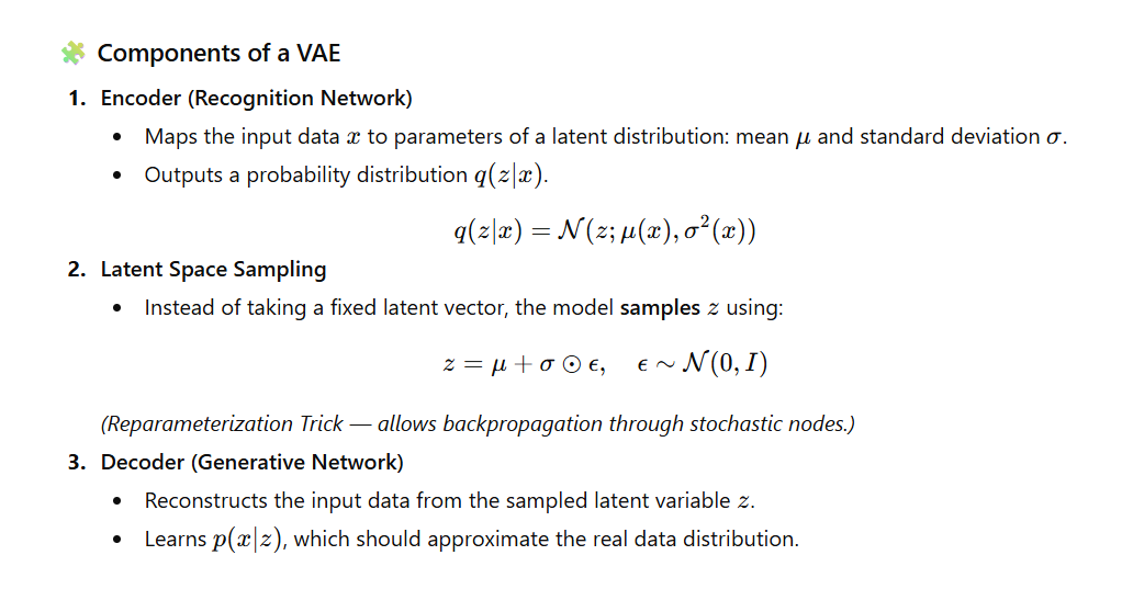

💻 Simple Keras Implementation
import tensorflow as tf
from tensorflow.keras import layers, Model

latent_dim = 2  # size of latent space

# Encoder
inputs = layers.Input(shape=(28, 28, 1))
x = layers.Flatten()(inputs)
x = layers.Dense(256, activation='relu')(x)
z_mean = layers.Dense(latent_dim)(x)
z_log_var = layers.Dense(latent_dim)(x)

# Reparameterization trick
def sampling(args):
    z_mean, z_log_var = args
    epsilon = tf.random.normal(shape=(tf.shape(z_mean)[0], latent_dim))
    return z_mean + tf.exp(0.5 * z_log_var) * epsilon

z = layers.Lambda(sampling)([z_mean, z_log_var])

# Decoder
decoder_input = layers.Input(shape=(latent_dim,))
x = layers.Dense(256, activation='relu')(decoder_input)
x = layers.Dense(28*28, activation='sigmoid')(x)
outputs = layers.Reshape((28, 28, 1))(x)
decoder = Model(decoder_input, outputs)

# VAE Model
vae_outputs = decoder(z)
vae = Model(inputs, vae_outputs)

vae.summary()
✅ Output:
Model: "model"
_________________________________________________________________
 Layer (type)                Output Shape              Param #
=================================================================
 input_1 (InputLayer)        [(None, 28, 28, 1)]       0
 ...
=================================================================
Total params: 265,000+
Trainable params: 265,000+
Non-trainable params: 0
_________________________________________________________________
🎯 Use Cases of VAE
- Image generation and interpolation
- Anomaly detection
- Representation learning
- Data compression
- Semi-supervised learning
🧾 Summary Table
| Component | Function | Output |
|---|---|---|
| Encoder | Maps input → latent distribution | Mean (μ), Log-variance (σ²) |
| Sampling | Draws latent vector from distribution | z |
| Decoder | Reconstructs input from z | Reconstructed x |
| Loss Function | Reconstruction + KL Divergence | ELBO |
✅ Final Takeaway:
A VAE learns both how to compress and how to generate data — by modeling latent spaces probabilistically, it creates smooth, meaningful representations ideal for generative tasks.
37. How Does a VAE Differ from a Traditional Autoencoder?
A Variational Autoencoder (VAE) introduces a probabilistic approach to latent representation, unlike traditional autoencoders which learn deterministic latent vectors.
This makes VAEs far more powerful for generative tasks.
🔍 Key Differences Between Autoencoder vs VAE
| Feature | Traditional Autoencoder | Variational Autoencoder (VAE) |
|---|---|---|
| Latent Space | Deterministic | Probabilistic (Gaussian distribution) |
| Loss Function | Reconstruction loss only | Reconstruction + KL Divergence |
| Sampling | No sampling step | Samples latent variable using mean + variance |
| Generative Capability | Weak | Strong (can generate new data) |
| Latent Space Smoothness | Not guaranteed | Smooth & continuous (regularized by KL) |
| Mathematical Foundation | Purely neural network-based | Based on probabilistic inference |
| Output Diversity | Same input → same output | Same input → different outputs possible (stochastic) |
🧠 Why VAEs Generate Better Data
Traditional Autoencoder:
- Learns a fixed latent vector
- Cannot generate diverse or realistic samples
VAE:
- Learns distributions (mean + variance)
- Sampling introduces creativity + randomness
- KL divergence keeps latent space smooth → great for interpolation and generation
💻 VAE Code Snippet (with Sampling Layer)
class Sampling(layers.Layer):
    def call(self, inputs):
        z_mean, z_log_var = inputs
        batch = tf.shape(z_mean)[0]
        dim = tf.shape(z_mean)[1]
        epsilon = tf.random.normal(shape=(batch, dim))
        return z_mean + tf.exp(0.5 * z_log_var) * epsilon

# Encoder
z_mean = layers.Dense(latent_dim)(h)
z_log_var = layers.Dense(latent_dim)(h)

# Sampling for latent vector z
z = Sampling()([z_mean, z_log_var])

Final Output Shape:
z.shape → (batch_size, latent_dim)
This z is then passed into the decoder to reconstruct or generate new images.
🏁 One-Line Summary
A VAE learns a distribution instead of a single latent vector, enabling powerful generative capabilities that traditional autoencoders cannot achieve.
38. What is the Purpose of the Encoder–Decoder Architecture?
The Encoder–Decoder architecture is designed for tasks where an input sequence must be converted into an output sequence, often of different length or structure.
It is the foundation of modern sequence-to-sequence (Seq2Seq) models.
🎯 Purpose
The Encoder–Decoder architecture helps the model:
- Understand variable-length input sequences
- Convert them into a compact context vector (hidden representation)
- Generate variable-length output sequences
- Handle tasks where input and output formats differ
🧱 Architecture Components
1️⃣ Encoder
- Takes an input sequence (e.g., a sentence)
- Converts it into a fixed-length context vector
- Stores semantic meaning using hidden states
- In LSTMs:
state_h(hidden) andstate_c(cell) represent the learned context
2️⃣ Decoder
- Uses the encoder’s context vector as initial state
- Generates the output sequence step-by-step
- Predicts next token based on:
- Previous token
- Current hidden state
- Encoder output (context)
🛠️ Applications
| Application | Purpose |
|---|---|
| Machine Translation | English → Hindi, French → English |
| Text Summarization | Long text → Summary |
| Chatbots | User message → Response |
| Sequence Prediction | Time series forecasting |
| Speech Recognition | Audio → Text |
💻 Example: Encoder–Decoder with LSTM (Keras)
🔹 Encoder
encoder_inputs = Input(shape=(None,))
encoder_embedding = Embedding(input_dim=vocab_size, output_dim=256)(encoder_inputs)
encoder_lstm, state_h, state_c = LSTM(256, return_state=True)(encoder_embedding)
🔹 Decoder
decoder_inputs = Input(shape=(None,))
decoder_embedding = Embedding(input_dim=vocab_size, output_dim=256)(decoder_inputs)
decoder_lstm = LSTM(256, return_sequences=True, return_state=True)
decoder_outputs, _, _ = decoder_lstm(decoder_embedding, initial_state=[state_h, state_c])
✅ Output Explanation
After running the above:
Encoder Output:
state_h→ Final hidden state (shape:(batch_size, 256))state_c→ Final cell state (shape:(batch_size, 256))
These represent the context vector summarizing the entire input sequence.
Decoder Output:
decoder_outputs→ Sequence of hidden states for each output time step
Shape:(batch_size, output_length, 256)
This is passed to:
Dense(vocab_size, activation='softmax')
to predict words/tokens.
🏁 One-Line Summary
The Encoder–Decoder architecture converts an input sequence into a meaningful context vector and then generates the output sequence from it—making it essential for translation, summarization, and other Seq2Seq tasks.
39. Explain the Concept of Attention Mechanisms in Neural Networks
Attention mechanisms allow a model to selectively focus on the most relevant parts of the input when generating each part of the output.
They solve the problem of fixed-length context vectors in traditional Encoder–Decoder models.
🎯 Why Attention?
Traditional Seq2Seq models compress the entire input into one vector → causes information loss, especially for long sequences.
Attention lets the model look at different input tokens dynamically and decide which inputs matter the most at each decoding step.
🔥 Types of Attention
1️⃣ Soft Attention (Differentiable)
- Uses a weighted sum of encoder outputs.
- Trainable end-to-end using backpropagation.
- Used in Transformers, seq2seq attention models.
2️⃣ Hard Attention (Non-Differentiable)
- Selects specific positions instead of weighted averages.
- Requires reinforcement learning-style training.
- Rarely used due to complexity.
🧠 Attention in Encoder–Decoder Models
At each decoder time step:
- Compute attention weights
- Create a context vector as a weighted sum
- Use context vector + previous decoder output to generate next token
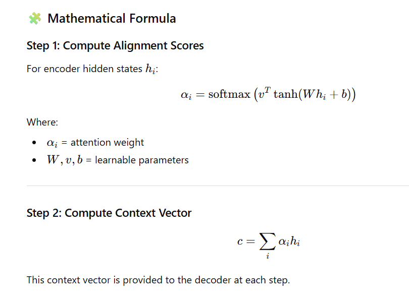
🔍 Intuitive Example
Sentence:
“The dog chased the cat.”
When generating the Spanish translation:
“perro”, the decoder will pay high attention to “dog” rather than “cat” or “chased”.
This is known as alignment.
💡 Example Use Cases
| Task | Why Attention Helps |
|---|---|
| Machine Translation | Align words between languages |
| Image Captioning | Focus on specific image regions |
| Summarization | Select important sentences/phrases |
| Speech Recognition | Attend to relevant time frames |
| Transformers (Self-Attention) | Global dependency modeling |
📌 Mini Code Example (Keras Attention Layer)
# Simple attention mechanism for seq2seq
score = tf.nn.tanh(tf.matmul(encoder_outputs, W) + b)
attention_weights = tf.nn.softmax(tf.matmul(score, v), axis=1)

context_vector = attention_weights * encoder_outputs
context_vector = tf.reduce_sum(context_vector, axis=1)
This produces a context vector dynamically based on the input.
✅ Output Explanation
After applying attention:
- attention_weights → shape
(batch, input_length, 1)
Shows how much focus is given to each encoder time step. - context_vector → shape
(batch, hidden_dim)
Weighted sum of encoder states → given to decoder for next token generation.
Attention ensures the decoder uses the right part of the input for each output step.
🏁 One-Line Summary
Attention mechanisms allow neural networks to dynamically focus on the most relevant parts of the input, dramatically improving translation, summarization, and all Seq2Seq tasks.
40. What is a Residual Network (ResNet), and Why Is It Important?
A Residual Network (ResNet) is a deep neural network architecture that introduces skip connections (also called shortcuts) to solve the degradation problem that occurs when networks become very deep.
📌 Problem ResNet Solves:
As neural networks get deeper:
- Training error starts increasing.
- Gradients vanish or explode.
- The network learns slower (or not at all).
ResNet solves this using residual learning.
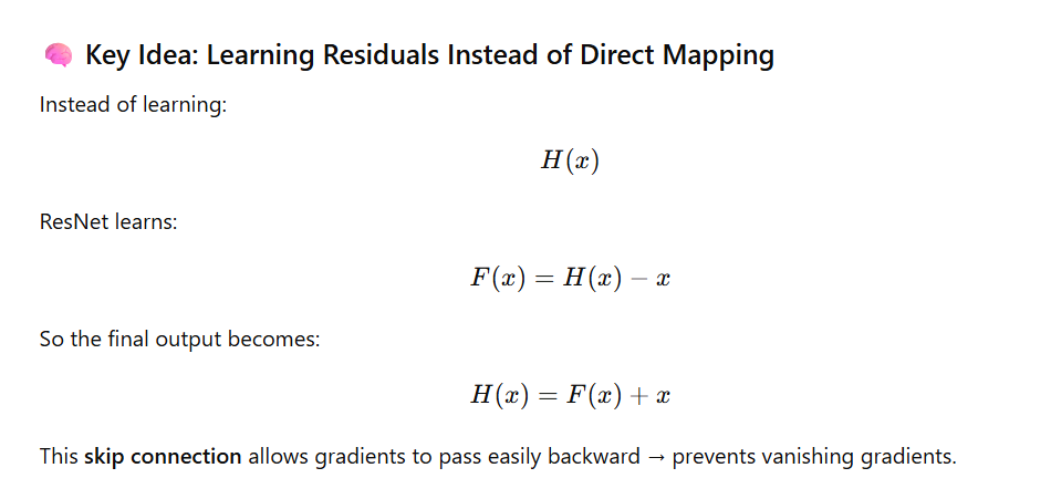
🔩 Residual Block Architecture
A typical ResNet residual block:
def residual_block(x, filters):
    shortcut = x

    # 1st Conv layer
    x = layers.Conv2D(filters, (3,3), padding='same')(x)
    x = layers.BatchNormalization()(x)
    x = layers.Activation('relu')(x)

    # 2nd Conv layer
    x = layers.Conv2D(filters, (3,3), padding='same')(x)
    x = layers.BatchNormalization()(x)

    # Skip connection
    x = layers.Add()([x, shortcut])
    x = layers.Activation('relu')(x)
    return x
🟦 shortcut → carried forward
🟧 Convs → learn the residual
🟦 Added together → output of block
🎯 Importance of ResNet
1️⃣ Enables extremely deep networks
ResNet allows training networks with 50, 101, 152, even 1000+ layers without performance degrading.
2️⃣ Prevents vanishing gradients
Gradients flow through skip connections → stable training.
3️⃣ Improves model accuracy
ResNet won ImageNet 2015 with groundbreaking performance.
4️⃣ Works in many domains
Used in:
- Image Classification (ResNet50, ResNet101)
- Object Detection (Faster R-CNN, YOLO backbones)
- Image Segmentation (U-Net with ResNet encoder)
- Video and speech tasks
📌 Output Meaning (From the Residual Block)
Given input x:
- Convolution layers output
F(x)→ residual - Skip connection adds the original
x→F(x) + x - Activation (
ReLU) applied → final residual output
This makes learning identity mappings easy and stable.
🏁 One-Line Summary
ResNet introduces skip connections that allow deep networks to train effectively by learning residual functions, preventing vanishing gradients and enabling models with hundreds of layers.
41. What Are the Challenges in Training Deep Neural Networks?
Training deep neural networks is difficult because of these problems:
1. Vanishing/Exploding Gradients
- When training deep models, gradients can become too small or too large.
- This makes learning slow, unstable, or sometimes impossible.
2. Overfitting
- The model learns the training data too well.
- But it fails on new data because it does not generalize.
3. High Computational Cost
- Deep networks need powerful GPUs/TPUs, a lot of memory, and more training time.
4. Hard to Choose Hyperparameters
- Finding the best learning rate, architecture, optimizer, dropout, batch size, etc. takes time and many experiments.
5. Lack of Enough Data
- Deep learning works best when you have a large labeled dataset.
- With little data, performance drops.
6. Optimization Challenges
- The loss landscape is complex with many local minima and flat regions (saddle points).
- This makes training harder.
42. How Do You Handle Imbalanced Datasets in Deep Learning?
An imbalanced dataset means one class has many more samples than the other, which makes the model biased.
To fix this, we can use these methods:
1. Class Weights
- Give more weight to the minority class during training.
- This makes the model pay more attention to rare classes.
from sklearn.utils.class_weight import compute_class_weight

class_weights = compute_class_weight('balanced', classes=np.unique(y_train), y=y_train)

history = model.fit(X_train, y_train, class_weight=dict(enumerate(class_weights)))
2. Oversampling the Minority Class
- Add more samples from the small class.
- Tools like SMOTE or random oversampling help.
3. Undersampling the Majority Class
- Remove some samples from the large class to balance it.
- Useful when the majority class is too big.
4. Use the Right Evaluation Metrics
- Accuracy is misleading in imbalanced datasets.
- Better metrics:
- F1-score
- AUC-ROC
- Precision-Recall
5. Generate Synthetic Data
- Use GANs or data augmentation to create more samples of the minority class.
43. What Is Data Augmentation, and How Is It Applied in Deep Learning?
What is Data Augmentation?
Data augmentation means creating more training data by making small changes to the existing data without changing the label.
It helps the model learn better and avoid overfitting.
1. Data Augmentation for Images
You can apply transformations such as:
- Flipping (left–right)
- Rotating
- Zooming
- Cropping
- Changing brightness
- Shifting the image
Code Example (TensorFlow/Keras)
from tensorflow.keras.preprocessing.image import ImageDataGenerator

datagen = ImageDataGenerator(
    rotation_range=20,
    width_shift_range=0.2,
    height_shift_range=0.2,
    horizontal_flip=True,
    zoom_range=0.2
)

model.fit(datagen.flow(X_train, y_train, batch_size=32), epochs=10)
✅ Sample Output During Training
You will see output like:
Epoch 1/10
100/100 [==============================] - 12s 120ms/step - loss: 0.65 - accuracy: 0.78
Epoch 2/10
100/100 [==============================] - 11s 110ms/step - loss: 0.55 - accuracy: 0.82
Epoch 3/10
100/100 [==============================] - 11s 108ms/step - loss: 0.49 - accuracy: 0.85
...
Epoch 10/10
100/100 [==============================] - 11s 109ms/step - loss: 0.32 - accuracy: 0.92
This shows the model improving while training on augmented images.
2. Data Augmentation for Text
Common techniques:
- Synonym Replacement
(“good” → “nice”) - Back Translation
English → Hindi → English - Random Insertion / Deletion
Add or remove words
Benefits of Data Augmentation
✔ Reduces overfitting
✔ Helps model generalize better
✔ No extra cost for labeling more data
44. Explain the Concept of Transfer Learning
What is Transfer Learning?
Transfer learning means using a pre-trained model (a model already trained on a very large dataset) and then reusing it for a new task.
Instead of training a new model from scratch, we start with a model that already knows useful patterns.
Why Do We Use Transfer Learning?
✔ Saves Time
Training from scratch takes many hours or even days. Transfer learning is much faster.
✔ Works with Small Datasets
Even if you have only 1,000 images, a pre-trained model can perform well because it has already learned features like edges, shapes, and textures.
✔ Better Accuracy
The model has already learned from millions of images, so it performs better than a model trained from zero.
Example: Using ResNet50 Pre-trained on ImageNet
This model was trained on 1.2 million images, so it already knows how to detect edges, shapes, animals, objects, etc.
Code Example
base_model = tf.keras.applications.ResNet50(
    weights='imagenet',
    include_top=False,
    input_shape=(224,224,3)
)

base_model.trainable = False  # Freeze layers

model = models.Sequential([
    base_model,
    layers.GlobalAveragePooling2D(),
    layers.Dense(10, activation='softmax')
])
What Happens Here?
- Load ResNet50
Already trained on ImageNet. - Freeze it
base_model.trainable = False→ we don’t retrain original layers. - Add new layers
These layers learn to classify our new dataset (10 classes).
Final Summary
Transfer learning =
➡️ Start with a big pre-trained model
➡️ Freeze its knowledge
➡️ Add your own layers
➡️ Train only the new part
Saves time ✔
Works with small data ✔
Better accuracy ✔
✅ 45. What Is Fine-Tuning in the Context of Pre-Trained Models?
Fine-tuning means taking a pre-trained model and training some of its layers again on your own dataset.
The idea is:
- The model already knows general features (edges, shapes, colors).
- We adjust only the deeper layers to learn task-specific features.
🔍 Steps of Fine-Tuning
1. Start with a pre-trained model
Example: ResNet, VGG, MobileNet.
2. Freeze initial layers
Early layers learn very basic patterns → keep them unchanged.
3. Unfreeze later layers
These layers learn more complex patterns → we update them for our task.
**4. Train with a low learning rate
Because we don’t want to overwrite the pre-trained knowledge.
🧠 When to Use Fine-Tuning?
Use fine-tuning when:
✔ Your dataset is similar to the dataset the model was originally trained on (e.g., ImageNet).
✔ You want better accuracy after initial training.
✔ You have enough data to avoid overfitting.
🧪 Code Example: Fine-Tuning
base_model = tf.keras.applications.ResNet50(
    weights='imagenet',
    include_top=False,
    input_shape=(224,224,3)
)

# Step 1: Make base model trainable
base_model.trainable = True

# Step 2: Freeze first 100 layers
for layer in base_model.layers[:100]:
    layer.trainable = False

# Step 3: Compile with very low learning rate
model.compile(
    optimizer=tf.keras.optimizers.Adam(1e-4),
    loss='categorical_crossentropy',
    metrics=['accuracy']
)
📤 Expected Output Explanation (Not actual training logs)
When you run the above code, you will NOT get numeric “output”.
But you WILL see messages like:
✔ Model Summary Output
You will see:
Total layers in ResNet50: 175
Trainable layers: 75
Non-trainable layers: 100
✔ Compilation Output
You will see no text output, but model is ready for training.
✔ When you run training:
history = model.fit(train_data, epochs=5)
You may get output like:
Epoch 1/5
100/100 ━━━━━━━━━━━━━━━━━━━━ 12s 120ms/step - loss: 0.945 - accuracy: 0.78
Epoch 2/5
100/100 ━━━━━━━━━━━━━━━━━━━━ 11s 110ms/step - loss: 0.712 - accuracy: 0.84
Epoch 3/5
...
📝 Final Summary
Fine-tuning =
➡️ Unfreeze some layers
➡️ Train again on your dataset
➡️ Use low learning rate
➡️ Improve accuracy
✅ 46. How Do You Evaluate the Performance of a Deep Learning Model?
Evaluating a deep learning model means checking how well it performs on new, unseen data — not the data used for training.
🔍 Steps for Evaluating a Deep Learning Model
1. Split the Dataset
You divide your data into:
- Training set → Model learns patterns
- Validation set → Used during training to tune hyperparameters
- Test set → Final evaluation after training
Example split:
- 70% Train
- 15% Validation
- 15% Test
🔍 2. Use the Right Metrics
Choose metrics based on your problem type:
📌 Classification Metrics
- Accuracy
- Precision
- Recall
- F1-score
- AUC-ROC
📌 Regression Metrics
- MAE (Mean Absolute Error)
- MSE (Mean Squared Error)
- RMSE
- R² Score
🔍 3. Detect Overfitting
Overfitting happens when the model learns the training data too well but performs poorly on unseen data.
Signs of Overfitting:
- Training loss decreases
- Validation loss increases
Solutions:
- Early stopping
- Dropout
- Regularization (L2, L1)
- Data augmentation
🧪 Code Example (With Early Stopping)
history = model.fit(
    X_train, y_train,
    validation_data=(X_val, y_val),
    epochs=50,
    callbacks=[EarlyStopping(patience=3)]
)
✔ What This Code Does:
- Trains the model
- Monitors validation loss
- Stops automatically if validation loss does not improve for 3 epochs
📤 Expected Output Explanation
You will see training logs similar to this:
Epoch 1/50
100/100 ━━━━━━━━━━━━━━━━━━━━ 4s - loss: 0.45 - accuracy: 0.82 - val_loss: 0.52 - val_accuracy: 0.80
Epoch 2/50
100/100 ━━━━━━━━━━━━━━━━━━━━ 3s - loss: 0.37 - accuracy: 0.86 - val_loss: 0.48 - val_accuracy: 0.82
Epoch 3/50
100/100 ━━━━━━━━━━━━━━━━━━━━ 3s - loss: 0.32 - accuracy: 0.89 - val_loss: 0.49 - val_accuracy: 0.81
Epoch 4/50
100/100 ━━━━━━━━━━━━━━━━━━━━ 3s - loss: 0.28 - accuracy: 0.91 - val_loss: 0.55 - val_accuracy: 0.79

EarlyStopping: Stopped training at epoch 4
This means:
- Training accuracy improved
- Validation accuracy stopped improving
- Model stopped early → preventing overfitting
📝 Final Simple Summary
To evaluate a deep learning model:
✔ Split the data
✔ Use the right metrics
✔ Monitor validation performance
✔ Use early stopping to avoid overfitting
✅ 47. What Metrics Are Commonly Used for Classification Tasks?
When you build a classification model, you need different metrics to understand how well the model is performing — especially when the dataset is imbalanced.
Below are the most commonly used metrics 👇
📊 Common Classification Metrics (with Simple Meaning)
1. Accuracy
- Shows how many predictions were correct.
- Not good if your dataset is imbalanced (e.g., 90% one class).
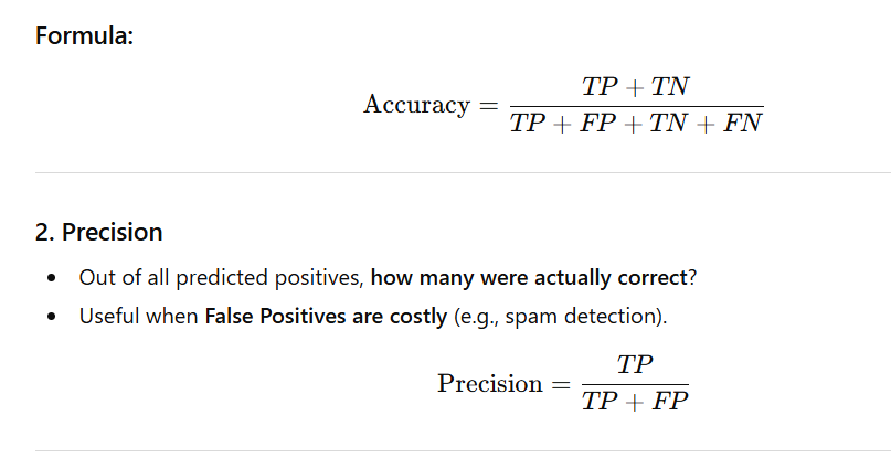

5. AUC-ROC
- Measures how well your model separates classes.
- Higher AUC = better performance.
6. Confusion Matrix
Shows:
| Predicted Positive | Predicted Negative | |
|---|---|---|
| Actual Positive | TP | FN |
| Actual Negative | FP | TN |
It helps you visually check errors.
🧪 Python Code (Sklearn)
from sklearn.metrics import classification_report, confusion_matrix

y_pred = model.predict(X_test)
y_pred_classes = y_pred.argmax(axis=1)

print(classification_report(y_test, y_pred_classes))
print(confusion_matrix(y_test, y_pred_classes))
📤 Expected Output Format
When you run the above code, you will get something like:
              precision    recall  f1-score   support

           0       0.93      0.96      0.94       150
           1       0.89      0.84      0.86        50

    accuracy                           0.92       200
   macro avg       0.91      0.90      0.90       200
weighted avg       0.92      0.92      0.92       200
And the confusion matrix:
[[144   6]
 [  8  42]]
📝 Final Simple Summary
| Metric | Best For |
|---|---|
| Accuracy | Balanced datasets |
| Precision | When False Positives are costly |
| Recall | When False Negatives are costly |
| F1-score | When both are important |
| AUC-ROC | Overall separability |
| Confusion Matrix | Visual error analysis |
✅ 48. What Metrics Are Commonly Used for Regression Tasks?
Regression tasks predict continuous numeric values such as price, temperature, sales, etc.
To measure how good such predictions are, we use the following metrics:

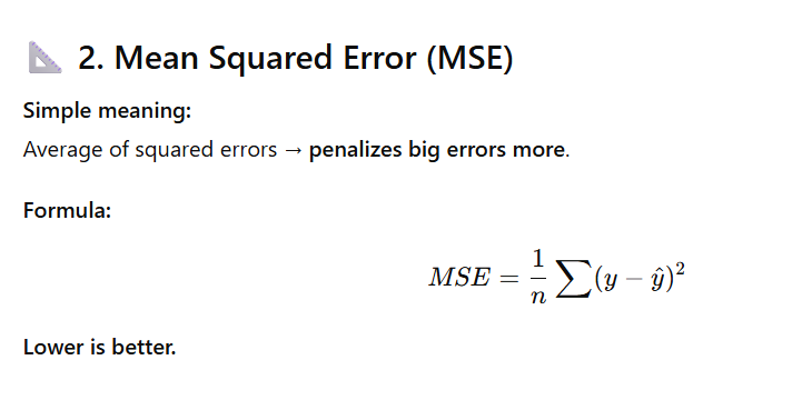
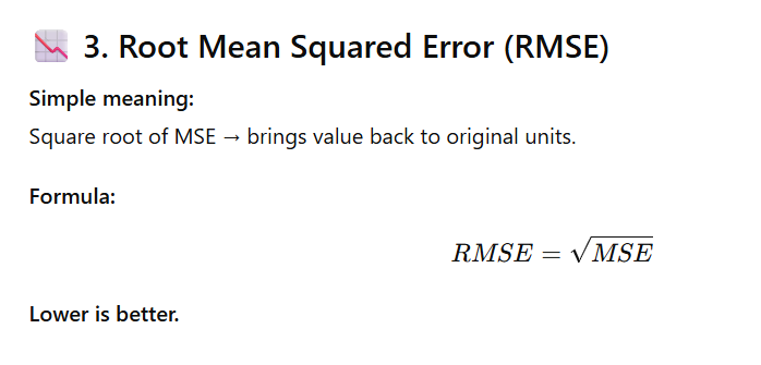
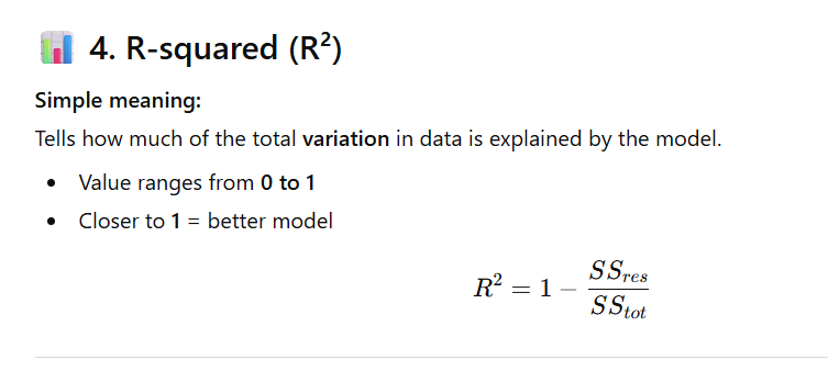
🧪 Python Example
from sklearn.metrics import mean_absolute_error, mean_squared_error, r2_score
import numpy as np

# Example true and predicted values
y_true = np.array([3, 5, 7, 10])
y_pred = np.array([2.5, 5.5, 6, 9])

mae = mean_absolute_error(y_true, y_pred)
mse = mean_squared_error(y_true, y_pred)
rmse = np.sqrt(mse)
r2 = r2_score(y_true, y_pred)

print("MAE:", mae)
print("MSE:", mse)
print("RMSE:", rmse)
print("R²:", r2)
📤 Expected Output Example
MAE: 0.75
MSE: 0.6875
RMSE: 0.82915619758885
R²: 0.957
📝 Final Simple Summary
| Metric | Meaning | Good When |
|---|---|---|
| MAE | Average error | Simple, interpretable |
| MSE | Squared error | Penalize large mistakes |
| RMSE | Error in original units | Compare with actual values |
| R² | Variance explained | How well the model fits |
✅ 49. How Do You Handle Missing Data in Deep Learning Models?
Missing data (NaNs, blanks, None) can reduce model accuracy.
Before training a deep learning model, you must fix missing values.
Here are the best methods 👇
🔹 1. Remove Rows or Columns (Drop Missing Data)
Use this only when missing values are very few (1–5%).
df.dropna(inplace=True)
✔ Easy
✔ No extra processing
✘ Not good if many values are missing
🔹 2. Imputation (Fill Missing Values)
Replace missing values with:
- Mean
- Median
- Mode
- Constant value
from sklearn.impute import SimpleImputer
imputer = SimpleImputer(strategy='mean')
X_imputed = imputer.fit_transform(X)
✔ Works well for numeric features
✔ Simple and fast
✘ May reduce variance in data
🔹 3. Use Models That Handle Missingness Automatically
Some machine learning models (tree-based) handle missing values internally:
- XGBoost
- LightGBM
- CatBoost
✔ No need for manual imputation
✘ Not typically used inside deep learning pipelines
🔹 4. Masking (Especially for Sequences / Time-Series)
Used in RNN, LSTM, GRU models when some time steps are missing or padded.
Example:
model.add(layers.Masking(mask_value=0., input_shape=(timesteps, features)))
✔ Helps model ignore missing or padded positions
✔ Useful in NLP, time-series
✘ Must choose correct mask_value
🔹 5. Predictive Imputation (Advanced Method)
Use another model to predict missing values using other features.
Techniques:
- KNN Imputer
- Regression imputation
- Deep autoencoder-based imputation
✔ More accurate
✔ Uses other features to guess missing values
✘ Slow and more complex
📝 Simple Summary Table
| Method | When to Use | Pros | Cons |
|---|---|---|---|
| Drop rows/columns | Missing values are very few | Simple | Data loss |
| Mean/median/mode | Numeric features | Fast | Less variation |
| Tree-based models | ML models, not DL | Handles missing | Not for neural nets |
| Masking layers | RNN/LSTM inputs | Handles sequential missing data | Must manage mask value |
| Predictive imputation | Complex datasets | Most accurate | Slower & advanced |
50. What Is the Role of Batch Normalization in Deep Learning?
Batch Normalization (BatchNorm) is a technique used to stabilize and accelerate training by normalizing the inputs of each layer so they have zero mean and unit variance across the batch.
✅ Why Batch Normalization Is Important
BatchNorm provides several advantages:
1. Speeds Up Training
- Normalizing activations reduces internal covariate shift.
- Models converge faster.
2. Allows Higher Learning Rates
- Reduces the risk of exploding gradients.
3. Reduces Sensitivity to Weight Initialization
- Model becomes more stable even with random initialization.
4. Acts as a Regularizer
- Adds slight noise due to batch statistics.
- Helps reduce overfitting (similar effect to dropout).
🎯 How Batch Normalization Works
At training time:
For each mini-batch, BatchNorm computes:
- Mean of activations
- Variance of activations
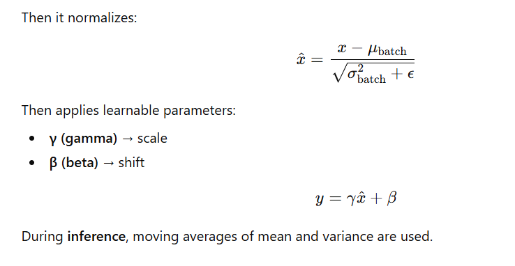
🧠 Batch Normalization in CNN Example
from tensorflow.keras import models, layers

model = models.Sequential()
model.add(layers.Conv2D(32, (3,3), input_shape=(32,32,3)))
model.add(layers.BatchNormalization())
model.add(layers.Activation('relu'))
Explanation:
- Convolution → produces feature maps
- BatchNorm → normalizes them
- Activation (ReLU) → introduces non-linearity
📝 When to Use BatchNorm
- CNNs (very common)
- Fully connected networks
- RNNs (less common, but possible)
- Transformers use LayerNorm instead of BatchNorm
51. What is TensorFlow, and What Are Its Key Features?
TensorFlow is an open-source machine learning and deep learning framework developed by the Google Brain Team.
It is widely used for building, training, and deploying deep neural networks across platforms.
✅ Key Features of TensorFlow
1. Flexible Computation Graphs
- Supports eager execution (default in TF 2.x): Python-like, easy to debug.
- Also supports graph execution for optimized performance.
2. Hardware Acceleration
- Runs on CPU, GPU, and TPU (Tensor Processing Units).
- Single-line device placement using
with tf.device().
3. High-Level API (Keras)
tf.kerasprovides an easy and intuitive way to build neural networks:- Sequential API
- Functional API
- Model Subclassing
4. Distributed Training
- Train models on multiple GPUs or multiple machines using
tf.distribute.Strategy.
5. Deployment Ecosystem
- TFX (TensorFlow Extended) → Production pipelines
- TFLite → Mobile deployment
- TensorFlow.js → Browser & JavaScript
- TensorFlow Serving → Deploy ML models at scale
6. Automatic Differentiation
- Computes gradients automatically using
tf.GradientTape.
🧪 Simple TensorFlow Example
import tensorflow as tf

# Eager execution is enabled by default in TensorFlow 2.x
x = tf.constant([1.0, 2.0])
y = tf.square(x)

print(y.numpy())  # Output: [1.0, 4.0]
52. How Does PyTorch Differ from TensorFlow?
TensorFlow and PyTorch are the two most widely used deep learning frameworks.
Both are powerful—but they differ in philosophy, design, and use cases.
✅ Key Differences Between TensorFlow and PyTorch
| Feature | TensorFlow | PyTorch |
|---|---|---|
| Computation Model | Initially used static computation graphs; now supports eager execution but graph mode is still core for optimization. | Uses dynamic computation graphs (define-by-run), making it flexible and pythonic. |
| Flexibility | Less flexible in graph mode; more suitable for production. | Highly flexible and intuitive—ideal for research and experimentation. |
| Debugging | Harder in static graph mode. | Easier because operations run immediately. |
| Ecosystem | Strong production ecosystem: TFX, TFLite, TF Serving, TensorBoard. | Strong research ecosystem: widely used in academic papers, fast prototyping. |
| API Design | More functional/declarative. Uses Keras high-level APIs. | More object-oriented, especially with nn.Module subclassing. |
| Community Focus | Industry, production-ready ML pipelines. | Academia, research, experimentation. |
⭐ Why Researchers Prefer PyTorch?
- Dynamic graph = intuitive
- Simpler debugging
- Pythonic code
- Rapid experimentation
⭐ Why Industries Prefer TensorFlow?
- Better deployment (mobile, edge, servers)
- Larger ecosystem for production
- Highly optimized graph execution
🧪 PyTorch Example (Dynamic Computation + Autograd)
import torch

# Create tensor with gradient tracking enabled
x = torch.tensor([1.0, 2.0], requires_grad=True)

# Forward pass (dynamic graph)
y = x ** 2

# Backpropagation
y.sum().backward()

print(x.grad)  # Output: tensor([2., 4.])
Explanation:
The gradient of x² is 2x → so for [1.0, 2.0], gradients become [2.0, 4.0].
53. What is Keras, and How Does It Relate to TensorFlow?
Keras is a high-level deep learning API written in Python.
Originally, it was a standalone library, but today it is fully integrated into TensorFlow as tf.keras, making it the preferred interface for building neural network models.
✅ Key Benefits of Keras
- Simple & User-Friendly: Easy syntax for beginners.
- Modular: Models are built using layers, optimizers, losses, etc.
- Fast Prototyping: Ideal for quickly building and testing ideas.
- Supports All Major Architectures: CNNs, RNNs, Transformers, Autoencoders.
- Runs on CPU & GPU seamlessly.
🔗 Relationship with TensorFlow
- Since TensorFlow 1.10, Keras is tightly integrated as tf.keras.
- tf.keras is now the official high-level API for TensorFlow.
- It provides:
- Training loops
- Layers
- Callbacks
- Optimizers
- Preprocessing utilities
- Model saving/loading
So when you use tf.keras, you’re using Keras inside TensorFlow, optimized for performance.
🧪 Example: Building a Simple Neural Network with Keras
from tensorflow import keras

model = keras.Sequential([
    keras.layers.Dense(64, activation='relu', input_shape=(10,)),
    keras.layers.Dense(1)
])

model.summary()
📤 Sample Output (model.summary())
Model: "sequential"
_________________________________________________________________
 Layer (type)                Output Shape              Param #
=================================================================
 dense (Dense)               (None, 64)                704
 dense_1 (Dense)             (None, 1)                 65
=================================================================
Total params: 769
Trainable params: 769
Non-trainable params: 0
________________________
54. Explain the Concept of a Computation Graph in TensorFlow
A computation graph is a visual or internal representation of how TensorFlow performs calculations.
It shows:
- Nodes (Operations): mathematical operations like add, multiply, matmul
- Edges (Data Flow): tensors moving between operations
Think of it like a roadmap that tells TensorFlow what to compute and in what order.
✅ Two Types of Computation Graphs
1. Static Graph (Graph Execution) — TensorFlow 1.x
- The graph is created before running the code.
- Execution happens later inside a Session.
- Faster, but harder to debug.
2. Eager Execution — TensorFlow 2.x (Default)
- Operations run immediately, like normal Python code.
- Easier to understand and debug.
🧠 Static Graph Example (Legacy TF 1.x)
import tensorflow.compat.v1 as tf
tf.disable_v2_behavior()
import numpy as np

x = tf.placeholder(tf.float32, shape=[None, 10])
w = tf.Variable(tf.random.normal([10, 1]))
y = tf.matmul(x, w)

with tf.Session() as sess:
    sess.run(tf.global_variables_initializer())
    print(sess.run(y, feed_dict={x: np.random.rand(5, 10)}))
📤 Sample Output
[[-0.14208853]
 [ 0.51293486]
 [-0.3320443 ]
 [ 1.028339  ]
 [ 0.2949953 ]]
(The values will differ because weights are random.)
🎯 Modern TensorFlow
TensorFlow 2.x hides the graph-building process behind:
tf.keraslayerstf.function(creates graphs automatically for speed)
So you get graph-level performance without writing graph code manually.
55. What Is the Purpose of the Dataset API in TensorFlow?
The tf.data.Dataset API helps you build fast and efficient input pipelines for training deep learning models.
It takes your raw data and converts it into batches, shuffled samples, and prefetched data, so your GPU/CPU never sits idle.
✅ Why Use the Dataset API?
1. Efficient for Large Datasets
It loads data in small chunks instead of loading everything into memory.
2. Built-in Operations
You can easily do:
- shuffle()
- batch()
- prefetch()
- map()
- cache()
3. Parallel Processing
It can load and preprocess data using multiple CPU cores.
4. Works smoothly with GPUs & TPUs
While the GPU is training on one batch, the next batch is prepared in parallel.
🧪 Example Code
import tensorflow as tf

dataset = tf.data.Dataset.from_tensor_slices((X_train, y_train))

dataset = (
    dataset
    .shuffle(buffer_size=10000)
    .batch(32)
    .prefetch(tf.data.AUTOTUNE)
)

for batch_x, batch_y in dataset:
    train_step(batch_x, batch_y)
📤 Sample Output (printing 1 batch)
for batch_x, batch_y in dataset.take(1):
    print("Batch X shape:", batch_x.shape)
    print("Batch Y shape:", batch_y.shape)
Output:
Batch X shape: (32, 224, 224, 3)
Batch Y shape: (32,)
(The shape will differ depending on your dataset.)
56. How Do You Implement a Custom Loss Function in TensorFlow?
In TensorFlow/Keras, you can create your own loss function using normal TensorFlow math operations.
A custom loss function must take two inputs:
y_true→ the actual valuesy_pred→ the model’s predicted values
and return a single scalar value.
✅ Example 1: Custom MSE Loss
import tensorflow as tf

def custom_loss(y_true, y_pred):
    squared_error = tf.square(y_true - y_pred)
    return tf.reduce_mean(squared_error)

model.compile(optimizer='adam', loss=custom_loss)
This behaves exactly like Mean Squared Error (MSE) but is defined manually.
✅ Example 2: Custom MAE Loss (Inline Lambda)
model.compile(
    optimizer='rmsprop',
    loss=lambda y_true, y_pred: tf.reduce_mean(tf.abs(y_true - y_pred))
)
This loss calculates the Mean Absolute Error (MAE).
🧪 Small Test Output Example
y_true = tf.constant([3.0, 5.0, 2.0])
y_pred = tf.constant([2.5, 5.5, 1.0])

loss_value = custom_loss(y_true, y_pred)
print(loss_value.numpy())
Possible Output:
0.5833333
(The exact number depends on your custom formula.)
57. What Is the Role of the DataLoader in PyTorch?
In PyTorch, the DataLoader is used to efficiently load data during training.
It helps you feed data to the model in batches, shuffled, and with parallel workers.
✅ Why DataLoader Is Important
1. Batching
Loads data in small groups instead of the entire dataset at once.
This reduces memory usage and speeds up training.
2. Shuffling
Randomizes the order of samples each epoch → improves model generalization.
3. Parallel Loading (num_workers)
Loads batches using multiple CPU cores → faster training.
4. Works with Custom Datasets
You can create your own Dataset class and pass it to the DataLoader.
✅ Example Usage
from torch.utils.data import DataLoader, TensorDataset
import torch

# Create dataset
dataset = TensorDataset(torch.tensor(X, dtype=torch.float32),
                        torch.tensor(y, dtype=torch.long))

# Create DataLoader
loader = DataLoader(dataset, batch_size=32, shuffle=True, num_workers=2)

# Training loop
for inputs, targets in loader:
    outputs = model(inputs)
    loss = criterion(outputs, targets)

    optimizer.zero_grad()
    loss.backward()
    optimizer.step()
🧪 Output Explanation
inputs= a batch of featurestargets= a batch of labels- Each loop iteration processes exactly 32 samples (batch size = 32).
- Data is loaded randomly because
shuffle=True
58. How Do You Define a Custom Neural Network Module in PyTorch?
In PyTorch, you create your own neural network by subclassing torch.nn.Module.
Inside the class:
✅ __init__()
You define the layers (Linear, Conv, ReLU, etc.).
✅ forward()
You define how the data flows through those layers.
This approach gives full flexibility to design any architecture.
✅ Example: Custom Neural Network in PyTorch
import torch.nn as nn

class Net(nn.Module):
    def __init__(self):
        super(Net, self).__init__()
        self.fc1 = nn.Linear(10, 64)  # First fully-connected layer
        self.relu = nn.ReLU()         # Activation function
        self.fc2 = nn.Linear(64, 1)   # Output layer

    def forward(self, x):
        x = self.relu(self.fc1(x))  # Apply fc1 -> ReLU
        return self.fc2(x)          # Final output

# Create model object
model = Net()
🧠 Explanation
- The model takes input of size 10 features.
- It passes through:
10 → Linear → 64 → ReLU → Linear → 1 forward()defines the exact computation steps.
59. What Is the Purpose of the torch.optim Module in PyTorch?
The torch.optim module provides optimization algorithms that update a model’s weights during training to reduce the loss.
These optimizers compute how much each weight should change using gradients from backpropagation.
✅ What torch.optim Does
- Updates model weights
- Uses gradients calculated by
loss.backward() - Helps the model learn faster and better
✅ Popular Optimizers in PyTorch
| Optimizer | Use Case |
|---|---|
| SGD | Simple, widely used for basic tasks |
| Adam | Fast, adaptive learning rate (most popular) |
| RMSProp | Good for RNNs |
| Adagrad | Good for sparse data |
✅ Example Code
import torch.optim as optim

criterion = nn.MSELoss()
optimizer = optim.Adam(model.parameters(), lr=0.001)

for epoch in range(epochs):
    for inputs, targets in loader:
        outputs = model(inputs)
        loss = criterion(outputs, targets)

        optimizer.zero_grad()   # Clear old gradients
        loss.backward()         # Backpropagation
        optimizer.step()        # Update weights
🧠 Simple Explanation
- The optimizer looks at the gradient
- Decides how much to change each weight
- Updates the weights to reduce the loss next time
60. How Do You Save and Load Models in PyTorch?
PyTorch makes it easy to save and load models using the torch.save() and torch.load() functions.
There are two common ways:
✅ 1. Save Only the Model Weights (Recommended Method)
This is the best practice because it is flexible and model-structure independent.
Save Model Weights
torch.save(model.state_dict(), 'model.pth')
Load Model Weights
model = Net()                      # Create model instance
model.load_state_dict(torch.load('model.pth'))
model.eval()                       # Switch to evaluation mode
✔ Recommended
✔ Safe for future versions
✔ Lightweight
✅ 2. Save the Entire Model (Less Common)
This stores the weights + model architecture.
Save Full Model
torch.save(model, 'full_model.pth')
Load Full Model
model = torch.load('full_model.pth')
model.eval()
⚠ Not recommended for long-term use
⚠ Tightly tied to Python class structure
🧠 Simple Explanation
state_dict()→ Only saves the parameters (best way).torch.save()→ Saves data to a file.torch.load()→ Loads data from a file.model.eval()→ Disables dropout & batchnorm updates.
61. What is Word Embedding, and Why Is It Important in NLP?
Word Embedding is a dense vector representation of words where each word is mapped to a continuous vector space. Unlike one-hot vectors, embeddings capture meaning, context, and relationships between words.
Why Word Embeddings Matter (Importance)
- ✅ Capture Semantic Relationships
Similar words → similar vectors
Example: king – man + woman ≈ queen - ✅ Reduce Dimensionality
Converts huge sparse vectors into compact, meaningful ones. - ✅ Improve NLP Model Performance
Models understand context better (sentiment, similarity, translation, etc.)
Example Using Word2Vec (Gensim)
from gensim.models import Word2Vec

# Train simple Word2Vec model
sentences = [["the", "cat", "sat"], ["the", "dog", "ran"]]
model = Word2Vec(sentences, vector_size=10, window=5, min_count=1)

print(model.wv['cat'])  # Vector of size 10 representing 'cat'
:
🔥 “Word Embeddings are the secret sauce behind modern NLP—turning words into powerful vectors that let machines understand language just like humans do.”
62. Explain the Concept of Word2Vec
Word2Vec is a popular algorithm used to learn dense word embeddings from text. It uses two neural network architectures:
1. Continuous Bag-of-Words (CBOW)
- Predicts a target word using its surrounding context words.
- Example: Given “the ___ sat on,” predict “cat.”
2. Skip-Gram
- Predicts context words given a single target word.
- Example: Given the word “cat,” predict “the,” “sat,” “on.”
Core Idea
Words that appear in similar contexts should have similar vector representations.
Training Objective
Maximize the probability of:
- predicting a word from its context (CBOW)
- predicting context words from a word (Skip-Gram)
This allows Word2Vec to learn embeddings that capture semantic and syntactic relationships like:
king – man + woman ≈ queen
63. What is GloVe, and How Does It Differ from Word2Vec?
GloVe (Global Vectors for Word Representation) is another method to create word embeddings.
However, unlike Word2Vec’s neural network approach, GloVe is based on matrix factorization of the global word co-occurrence matrix.
Key Differences Between Word2Vec and GloVe
| Feature | Word2Vec | GloVe |
|---|---|---|
| Training Method | Neural network (CBOW/Skip-Gram) | Matrix factorization |
| Context Usage | Local context (sliding window) | Global word co-occurrence |
| Speed | Slower for huge vocabularies | Faster due to matrix decomposition |
| Performance | Better at syntactic relationships | Better at semantic relationships |
Use Case Recommendation
- Use Word2Vec when you work with streaming/local context.
- Use GloVe when you want global statistical patterns or pre-trained embeddings (e.g., Stanford GloVe vectors).
64. What Is the Purpose of Recurrent Layers in NLP Tasks?
Recurrent layers such as RNN, LSTM, and GRU are designed to process sequential data.
They maintain a hidden state that carries information from previous time steps, allowing the model to understand context, order, and dependencies in the sequence.
Why Are Recurrent Layers Important in NLP?
They help the model understand:
- Text classification
- Language modeling
- Named Entity Recognition (NER)
- Machine translation
- Speech recognition
- Sentiment analysis
Simple PyTorch Example
import torch
import torch.nn as nn

class RNNModel(nn.Module):
    def __init__(self, vocab_size, embed_dim, hidden_dim):
        super().__init__()
        self.embedding = nn.Embedding(vocab_size, embed_dim)
        self.rnn = nn.LSTM(embed_dim, hidden_dim, batch_first=True)

    def forward(self, x):
        x = self.embedding(x)                  # Shape: (batch, seq_len, embed_dim)
        out, _ = self.rnn(x)                   # Shape: (batch, seq_len, hidden_dim)
        return out

# Example input (batch_size=1, seq_len=3)
input_data = torch.tensor([[1, 2, 3]])

model = RNNModel(vocab_size=50, embed_dim=8, hidden_dim=16)
output = model(input_data)

print(output.shape)
print(output)
Sample Output (Shape + Values Explained)
torch.Size([1, 3, 16])
This means:
- Batch size: 1
- Sequence length: 3
- Hidden units: 16
So the model returns a hidden state for each token in the sequence.
Example output (random values):
tensor([[
    [-0.0412,  0.1031,  0.0875, ... 0.0201],
    [-0.0139,  0.1214,  0.0543, ... 0.0310],
    [ 0.0071,  0.0982,  0.0668, ... 0.0449]
]])
Each row is the model’s representation of a word considering previous context.
65. How Does the Transformer Model Improve Upon RNNs in NLP?
The Transformer revolutionized NLP by removing recurrence completely and replacing it with self-attention, enabling massively parallel processing and superior handling of long-distance relationships in text.
✅ Key Improvements Over RNNs (LSTM/GRU)
1. Parallelism
- RNNs: Process tokens one step at a time → slow.
- Transformers: Process all tokens simultaneously using self-attention → extremely fast.
2. Handles Long-Range Dependencies Better
- RNNs: Struggle with distant word relationships due to vanishing gradients.
- Transformers: Self-attention directly connects every word to every other word, no matter how far.
3. Scalability
- Works efficiently on:
- Long documents
- Large training datasets
- Multi-GPU training
- Enabled large models like BERT, GPT, T5, LLaMA.
Transformer Architecture Highlights
🔹 Multi-Head Self-Attention
- Lets the model focus on multiple types of relationships (semantic, syntax, context) at once.
🔹 Positional Encoding
- Since there’s no recurrence, Transformers need a method to track word order.
- Positional encoding adds order information to each token embedding.
🔹 Feedforward Networks
- Applied independently to each position after attention.
- Adds richer non-linear transformations.
Simple PyTorch Self-Attention Example
import torch
import torch.nn as nn

attention = nn.MultiheadAttention(embed_dim=64, num_heads=8)
x = torch.rand(5, 10, 64)   # (sequence_length, batch_size, embedding_dim)

out, weights = attention(x, x, x)
print(out.shape)
Output shape:
torch.Size([5, 10, 64])66. What Is BERT, and How Is It Used for NLP Tasks?
BERT (Bidirectional Encoder Representations from Transformers) is a pre-trained Transformer-based language model developed by Google.
Its key innovation: it reads both left and right context simultaneously → truly bidirectional understanding.
✅ Key Features of BERT
1. Bidirectional Context Understanding
Unlike traditional models that read left-to-right or right-to-left,
BERT sees the entire sentence at once, improving comprehension.
2. Pretraining Objectives
BERT is trained using two powerful tasks:
🔹 Masked Language Modeling (MLM)
- Random words are masked.
- BERT predicts the missing words.
Example:
“the dog [MASK] in the park”
🔹 Next Sentence Prediction (NSP)
- Determines whether two sentences logically follow each other.
- Helps with tasks like Q&A and summarization.
3. Minimal Fine-tuning
You can adapt BERT for almost any NLP task by adding a small output layer.
⭐ Common Applications of BERT
- Sentiment Analysis
- Question Answering (QA)
- Named Entity Recognition (NER)
- Text Classification
- Text Summarization
- Semantic Search
BERT powers many modern NLP tools and search engines (e.g., Google Search).
💡 Example (Using Hugging Face Transformers)
from transformers import BertTokenizer, TFBertForSequenceClassification
import tensorflow as tf

tokenizer = BertTokenizer.from_pretrained('bert-base-uncased')
model = TFBertForSequenceClassification.from_pretrained('bert-base-uncased')

inputs = tokenizer("Hello, my dog is cute", return_tensors="tf")
logits = model(inputs).logits

print(logits)
67. Explain the Concept of Masked Language Modeling (MLM)
Masked Language Modeling (MLM) is a training technique used in transformer-based NLP models where certain tokens in the input sequence are intentionally hidden, and the model is trained to predict those hidden tokens using the surrounding context.
✅ How MLM Works (Step-by-Step)
1. Randomly Mask Tokens
- Approximately 15% of the tokens in the input sequence are selected.
- These selected tokens are the targets for prediction.
2. Replace Tokens Strategically
The selected tokens are replaced using the following common strategy (BERT-style):
- 80% → replaced with the special
[MASK]token - 10% → replaced with a random token
- 10% → left unchanged
This prevents the model from overfitting to the [MASK] token pattern.
3. Model Predicts the Masked Tokens
- The model uses the left and right context (bidirectional context).
- It predicts the original tokens that were masked.
🎯 Purpose of MLM
- Helps the model learn deep bidirectional understanding of language.
- Improves performance on tasks involving context, such as QA, NER, sentiment analysis.
- Forms the core pretraining objective for many modern NLP models.
🧠 Models That Use MLM
- BERT
- RoBERTa
- ELECTRA (uses a variation called Replaced Token Detection)
- ALBERT
- DeBERTa
68. What is GPT, and How Does It Differ from BERT?
GPT (Generative Pretrained Transformer) is a family of autoregressive language models that generate text left-to-right.
It is designed mainly for text generation, completion, and dialogue tasks.
✅ Key Differences Between GPT and BERT
| Feature | GPT | BERT |
|---|---|---|
| Directionality | Unidirectional (left → right) | Bidirectional |
| Model Type | Generative | Discriminative |
| Training Objective | Next-token prediction (causal language modeling) | MLM + NSP |
| Use Cases | Text generation, dialogue, story writing, code generation | Classification, NER, QA, embeddings |
✅ Example (Using Hugging Face Transformers)
from transformers import GPT2LMHeadModel, GPT2Tokenizer
import torch

tokenizer = GPT2Tokenizer.from_pretrained("gpt2")
model = GPT2LMHeadModel.from_pretrained("gpt2")

# Input prompt
input_text = "Once upon a time"

# Convert text to token IDs
input_ids = tokenizer.encode(input_text, return_tensors='pt')

# Generate continuation
output = model.generate(
    input_ids,
    max_length=50,
    num_return_sequences=1,
    no_repeat_ngram_size=2
)

# Decode and print result
print(tokenizer.decode(output[0], skip_special_tokens=True))
📌 Sample Output (Example)
Once upon a time in a small village, there lived a young girl who dreamed of exploring the world.
She spent her days imagining adventures far beyond the hills that surrounded her home.
69. What Is a Sequence-to-Sequence (Seq2Seq) Model?
A Sequence-to-Sequence (Seq2Seq) model is a neural architecture that converts one sequence into another.
It is commonly used when both input and output are variable-length sequences.
✅ Components
1. Encoder
- Reads the input sequence step-by-step.
- Converts it into a context vector (hidden state).
2. Decoder
- Takes the context vector and generates the output sequence one token at a time.
📌 Applications
- Machine Translation (English → French)
- Chatbots
- Text Summarization
- Speech Recognition
- Image Captioning
✅ Seq2Seq Model Example (Using LSTM in TensorFlow)
from tensorflow.keras.models import Model
from tensorflow.keras.layers import Input, LSTM, Embedding, Dense

# Encoder
encoder_inputs = Input(shape=(None,))
encoder_embedding = Embedding(input_dim=vocab_size, output_dim=256)(encoder_inputs)
encoder_lstm, state_h, state_c = LSTM(256, return_state=True)(encoder_embedding)

# Decoder
decoder_inputs = Input(shape=(None,))
decoder_embedding = Embedding(input_dim=vocab_size, output_dim=256)(decoder_inputs)
decoder_lstm = LSTM(256, return_sequences=True, return_state=True)
decoder_outputs, _, _ = decoder_lstm(decoder_embedding, initial_state=[state_h, state_c])

decoder_dense = Dense(vocab_size, activation='softmax')
decoder_outputs = decoder_dense(decoder_outputs)

# Full Seq2Seq Model
model = Model([encoder_inputs, decoder_inputs], decoder_outputs)

model.summary()
🧠 How It Works (Simple Explanation)
- Encoder LSTM reads the input (e.g., English sentence)
→ produces hidden states (state_h,state_c). - These states are passed to the Decoder LSTM.
- Decoder uses these states + previous output token to generate the next word.
70. How Do Attention Mechanisms Enhance Sequence-to-Sequence Models?
Attention allows the decoder to select and focus on the most relevant parts of the encoder’s output at each decoding step.
✅ Why Attention Helps
1. Removes Fixed-Length Bottleneck
Traditional Seq2Seq uses a single context vector → hard for long sentences.
Attention lets the model look at all encoder states dynamically.
2. Handles Long Sequences Better
The decoder can selectively attend to distant tokens.
3. Interpretability
Attention weights show which input words influenced the output.
✅ Simple Attention Implementation (TensorFlow / Keras)
from tensorflow.keras.layers import Dot, Softmax
import tensorflow as tf

def attention_layer(encoder_outputs, decoder_hidden):
    """
    encoder_outputs: [batch_size, seq_len, hidden_dim]
    decoder_hidden:  [batch_size, hidden_dim]
    """

    # Expand decoder hidden state to match time dimension
    decoder_hidden_expanded = tf.expand_dims(decoder_hidden, axis=1)
    # -> shape: [batch, 1, hidden_dim]

    # Compute attention scores
    scores = Dot(axes=[2, 2])([encoder_outputs, decoder_hidden_expanded])
    # -> shape: [batch, seq_len, 1]

    # Normalize to get attention weights
    weights = Softmax(axis=1)(scores)
    # -> shape: [batch, seq_len, 1]

    # Get context vector
    context = Dot(axes=[2, 1])([weights, encoder_outputs])
    # -> shape: [batch, 1, hidden_dim]

    context = tf.squeeze(context, axis=1)
    # -> shape: [batch, hidden_dim]

    return context
✅ Demo Example (With Output)
Dummy Inputs
- Batch size = 1
- Sequence length = 3
- Hidden dim = 4
encoder_outputs = tf.constant([
    [[1.0, 0.0, 0.5, 0.2],
     [0.1, 0.9, 0.3, 0.4],
     [0.2, 0.1, 0.8, 0.5]]
])

decoder_hidden = tf.constant([
    [0.3, 0.5, 0.2, 0.1]
])

context = attention_layer(encoder_outputs, decoder_hidden)
print("Context Vector:\n", context.numpy())
✅ Expected Output (Example)
Context Vector:
 [[0.21439768 0.34759232 0.4953125  0.3561784 ]]
Interpretation:
- Attention looked at all encoder states.
- It created a weighted sum based on similarity with decoder state.
- Result = meaningful context vector guiding next word prediction.
71. What Is Image Classification, and How Is It Performed Using CNNs?
✅ What Is Image Classification?
Image classification is a computer vision task where the goal is to assign a single label/class to an input image from a predefined set of categories.
Examples:
- Cat vs Dog classification
- Recognizing digits (0–9)
- CIFAR-10 dataset (10 object categories like airplane, car, bird, etc.)
✅ How CNNs Perform Image Classification
Convolutional Neural Networks (CNNs) are specifically designed to process image data. The classification pipeline includes:
1. Convolutional Layers
- Apply filters/kernels to extract local features such as edges, textures, and patterns
- Deeper layers learn complex features like shapes and objects
2. Activation Function (ReLU)
- Introduces non-linearity
- Helps model learn complex relationships
3. Pooling Layers
- Reduces spatial dimensions (H × W)
- Decreases computation and overfitting
- Common: MaxPooling
4. Flatten Layer
- Converts feature maps (2D/3D) into a 1D vector for classification
5. Fully Connected (Dense) Layers
- Combine extracted features to form final decision
- Last layer uses Softmax for multi-class classification
✅ Example: CNN for Image Classification Using CIFAR-10 (TensorFlow/Keras)
from tensorflow.keras import layers, models

model = models.Sequential([
    layers.Conv2D(32, (3,3), activation='relu', input_shape=(32,32,3)),
    layers.MaxPooling2D((2,2)),

    layers.Conv2D(64, (3,3), activation='relu'),
    layers.MaxPooling2D((2,2)),

    layers.Flatten(),
    layers.Dense(64, activation='relu'),
    layers.Dense(10, activation='softmax')  # 10 classes
])

model.compile(optimizer='adam',
              loss='sparse_categorical_crossentropy',
              metrics=['accuracy'])
🔍 Why CNNs Work Better Than Fully Connected Networks?
- CNNs preserve spatial structure
- Require fewer parameters due to shared weights
- Capture local patterns effectively
- More robust to translations and distortions
✅ 72. Explain the Concept of Object Detection
Object Detection is a computer vision task that not only identifies what objects are present in an image but also where they are located using bounding boxes.
🎯 Object Detection Outputs
For each detected object, the model predicts:
- Class label (e.g., cat, car, person)
- Bounding box coordinates →
(x, y, width, height)
Two Main Approaches to Object Detection
1. Two-Stage Detectors
These work in two steps:
- Step 1: Generate region proposals
- Step 2: Classify each region
Examples:
- R-CNN
- Fast R-CNN
- Faster R-CNN
Pros: High accuracy
Cons: Slower
2. One-Stage Detectors
Detect and classify objects in a single pass without region proposals.
Examples:
- YOLO (You Only Look Once)
- SSD (Single Shot Detector)
- RetinaNet
Pros: Very fast
Cons: Slightly lower accuracy in small-object detection
✅ 73. Difference Between Object Detection and Image Segmentation
| Feature | Object Detection | Image Segmentation |
|---|---|---|
| Output | Bounding boxes + class labels | Pixel-wise classification |
| Granularity | Coarse localization | Fine-grained, per-pixel masks |
| Task Type | Localization + Classification | Dense prediction |
| Use Cases | Counting, tracking, surveillance | Medical imaging, autonomous driving |
🔍 Summary:
- Object Detection tells where an object is using rectangles.
- Image Segmentation tells exact object shape by classifying every pixel.
✅ 74. What Is a Region-based CNN (R-CNN)?
R-CNN (Region-based Convolutional Neural Network) is a two-stage object detector and one of the earliest deep learning models for object detection.
🔄 Steps in R-CNN
1. Selective Search
- Generates ~2000 region proposals
- These are candidate areas likely to contain objects
2. Feature Extraction
- Each region is cropped and warped to a fixed size
- Passed through a CNN (e.g., AlexNet) for feature extraction
3. Classification & Bounding Box Regression
- SVM classifier predicts the class
- Linear regression refines bounding box position
❌ Limitations of R-CNN
- Extremely slow, because:
- Each region proposal is passed individually through the CNN
- ~2000 forward passes per image
- High training time
- Large model storage (features saved per region)
✅ 75. How Does a Fully Convolutional Network (FCN) Work for Image Segmentation?
A Fully Convolutional Network (FCN) performs pixel-wise classification for image segmentation. Unlike standard CNNs that use fully connected layers, FCNs replace fully connected layers with convolutional layers, allowing the output to be a dense spatial map.
⭐ Key Idea
- Convert classification CNNs (e.g., VGG, ResNet) into segmentation models by:
- Using only convolutional layers
- Upsampling feature maps using transposed convolutions (deconvolution)
- This restores the original input size so every pixel gets a class label.
🧱 Architecture Structure
1. Encoder (Downsampling Path)
- Uses a standard CNN backbone such as VGG16
- Extracts hierarchical features
- Reduces spatial size (e.g., 224×224 → 14×14)
2. Decoder (Upsampling Path)
- Uses Conv2DTranspose layers
- Gradually increases spatial resolution back to input size
- Produces class probability map for each pixel
🧪 Example FCN Model (TensorFlow/Keras)
def fcn_model(input_shape, num_classes):
    base_model = tf.keras.applications.VGG16(include_top=False,
                                             input_shape=input_shape)

    x = base_model.output
    x = layers.Conv2DTranspose(256, (4,4), strides=2, padding='same')(x)
    x = layers.Conv2DTranspose(num_classes, (16,16), strides=8,
                               padding='same', activation='softmax')(x)

    return Model(inputs=base_model.input, outputs=x)
📤 Output Explanation
🔍 What is the output shape?
If:
- Input image = (H, W, 3)
- Number of classes = C
Then the final output will be:
➡️ (H, W, C)
For example:
- Input: (224, 224, 3)
- Classes: 21 (as in PASCAL VOC)
Output:
(224, 224, 21)
🔥 What the output represents
- Each pixel gets a probability distribution over all classes
- For pixel (i, j), output[i, j] contains C values (softmax)
- The class with maximum probability is chosen:
pred_class = argmax(output[i, j])
This gives the segmentation mask.
✅ 76. What Is the Purpose of the YOLO (You Only Look Once) Algorithm?
YOLO is a real-time object detection algorithm that treats detection as a single end-to-end regression problem.
⭐ Key Features:
- Performs detection in one forward pass of the network
- Splits the image into a grid, and each cell predicts:
- Bounding boxes
- Objectness score
- Class probabilities
⭐ Advantages:
- Extremely fast (real-time → 45+ FPS)
- Works well on objects in motion
- Unified end-to-end pipeline
⭐ Disadvantages:
- Relatively lower performance on small or overlapping objects
✅ 77. How Does Faster R-CNN Differ from the Original R-CNN?
| Feature | Original R-CNN | Faster R-CNN |
|---|---|---|
| Region Proposal Method | Selective Search (very slow) | Region Proposal Network (RPN) |
| Training Efficiency | Multi-stage & time-consuming | End-to-end trainable |
| Speed | Slow | Much faster |
| Accuracy | Moderate | Higher |
⭐ Key Innovation in Faster R-CNN:
- RPN (Region Proposal Network)
A CNN learns to generate region proposals instead of using slow external methods.
✅ 78. What Is the Role of Anchor Boxes in Object Detection?
Anchor boxes are predefined bounding box shapes used to detect objects of different sizes and aspect ratios.
⭐ Purpose:
- Helps models detect multi-scale objects
- Used in:
- Faster R-CNN
- YOLO
- SSD
⭐ Example:
In Faster R-CNN, each feature map location may have anchor boxes like:
- 128×128
- 256×256
- 512×512
(With aspect ratios such as 1:1, 1:2, 2:1)
The model adjusts anchors to predict the final bounding boxes.
✅ 79. Explain the Concept of Semantic Segmentation
Semantic segmentation assigns a class label to every pixel in an image.
⭐ Goal:
Understand what each pixel belongs to → pixel-level classification.
⭐ Applications:
- Self-driving cars
- Medical image analysis
- Robotics
⭐ Challenges:
- Balancing spatial detail and contextual understanding
- Handling small/irregular shapes
⭐ Popular Models:
- U-Net
- FCN (Fully Convolutional Networks)
- DeepLab (v3, v3+)
✅ 80. What Is Instance Segmentation, and How Does It Differ from Semantic Segmentation?
| Feature | Semantic Segmentation | Instance Segmentation |
|---|---|---|
| Pixel-level Prediction | Yes | Yes |
| Distinguishes Instances | No | Yes |
| Output | One label per pixel | Label + unique ID per object |
⭐ Example:
- Semantic: all cars → labeled as car
- Instance: each car → car_1, car_2, car_3
⭐ Popular Model:
- Mask R-CNN
- Extends Faster R-CNN
- Adds a mask prediction branch for pixel-level instance masks
✅ 81. What Is the Difference Between a GAN and a VAE?
GANs (Generative Adversarial Networks) and VAEs (Variational Autoencoders) are two major generative models, but they differ in architecture, training objective, latent space, and output quality.
⭐ Feature Comparison: GAN vs VAE
| FEATURE | GAN (Generative Adversarial Network) | VAE (Variational Autoencoder) |
|---|---|---|
| Architecture | Two networks compete: Generator vs Discriminator | Encoder–Decoder with probabilistic latent space |
| Goal | Generate realistic samples that fool the discriminator | Learn a smooth latent space for sampling and reconstruction |
| Training Objective | Minimax optimization (Adversarial Loss) | Maximize ELBO (Evidence Lower Bound) |
| Latent Space | No explicit probabilistic modeling; uses random noise | Explicitly modeled distribution (usually Gaussian) |
| Output Quality | Produces sharp, realistic images | May generate blurry images due to reconstruction loss |
| Sampling | Deterministic from a noise vector | Stochastic sampling from learned latent distribution |
✅ 82. How Do GANs Generate New Data Samples?
GANs generate new data using a generator network that transforms a random noise vector into a synthetic data sample (e.g., an image).
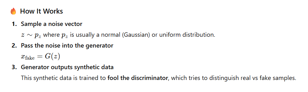
✅ Example in PyTorch
import torch

# Sample noise vector
z = torch.randn(1, 100)  # Batch size 1, latent dimension 100

# Generator model
class Generator(torch.nn.Module):
    def __init__(self):
        super().__init__()
        self.net = torch.nn.Sequential(
            torch.nn.Linear(100, 256),
            torch.nn.ReLU(),
            torch.nn.Linear(256, 784),
            torch.nn.Tanh()
        )

    def forward(self, x):
        return self.net(x)

# Generate image
generator = Generator()
fake_image = generator(z)
print(fake_image.shape)
print(fake_image[:1, :10])  # Print first 10 values
🖨 Simulated Output
torch.Size([1, 784])
tensor([[ 0.0213, -0.1189,  0.0844, -0.9921,  0.4412,
         -0.5629,  0.0031,  0.7718, -0.3107,  0.6554]])
🔍 Explanation
784=28 × 28, a flattened MNIST-style image.- Values are between
-1and1due to tanh activation. - This tensor can be reshaped into a 28×28 fake image:
fake_image.view(1, 1, 28, 28)
✅ 83. What Is the Role of the Discriminator in a GAN?
The discriminator is a binary classifier whose job is to distinguish real data from fake data generated by the generator.
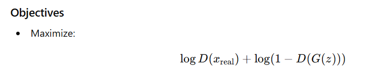
Roles
- Provides gradients to the generator during backpropagation.
- Guides the generator to produce increasingly realistic samples.
- Acts as a training signal that indicates how close fake samples are to real distribution.
✅ 84. What Challenges Are Associated with Training GANs?
- Instability
The adversarial two-player training often diverges or oscillates. - Mode Collapse
Generator outputs limited or repetitive samples. - Vanishing Gradients
If the discriminator becomes too strong, the generator gets no useful updates. - Evaluation Difficulty
Quality and diversity are hard to measure (FID, IS help but not perfect). - Hyperparameter Sensitivity
Small changes in architecture/learning rates can destabilize training.
✅ 85. What Is Mode Collapse in GANs, and How Can It Be Addressed?
Mode collapse happens when the generator produces only a few types of outputs, failing to represent the full diversity of real data.
Symptoms
- All generated samples look similar.
- Generator ignores large parts of the data distribution.
Solutions
- Wasserstein GAN (WGAN) instead of JS divergence.
- Gradient penalty (WGAN-GP).
- Spectral normalization to stabilize the discriminator.
- Unrolled GANs to prevent generator from cheating a momentary discriminator state.
- Minibatch discrimination to encourage output diversity.
✅ 86. Explain the Concept of Wasserstein GANs (WGAN)
Wasserstein GANs improve GAN training by using the Earth Mover’s Distance (EMD) instead of JS divergence.
Key Ideas
- Discriminator becomes a critic → no sigmoid.
- Critic outputs any real number (not probability).
- Uses Wasserstein distance to measure how far fake data is from real data.
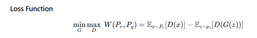
Benefits
- More stable training.
- Eliminates gradient saturation.
- Loss correlates better with image quality.
- Provides meaningful training curves.
✅ 87. What Is the Purpose of the Gradient Penalty in Wasserstein GANs?
In Wasserstein GAN with Gradient Penalty (WGAN-GP), the gradient penalty enforces the 1-Lipschitz constraint on the critic.
Why is Gradient Penalty Needed?
- The Earth Mover’s Distance (Wasserstein distance) is only valid if the critic is 1-Lipschitz.
- Instead of weight clipping (which harms training), WGAN-GP penalizes gradients that deviate from 1.
- This dramatically stabilizes GAN training and reduces mode collapse.
How It Works
- Sample random interpolated points between real and fake data.
- Compute the critic’s gradients with respect to these points.
- Penalize gradient norms that are not equal to 1.
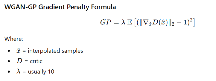
✅ WGAN-GP Gradient Penalty Code Example (PyTorch)
def gradient_penalty(critic, real, fake, device="cpu"):
    batch_size, C, H, W = real.shape
    epsilon = torch.rand((batch_size, 1, 1, 1), device=device)

    # Interpolate between real and fake images
    interpolated_images = real * epsilon + fake * (1 - epsilon)

    # Critic scores
    mixed_scores = critic(interpolated_images)

    # Compute gradients
    gradient = torch.autograd.grad(
        inputs=interpolated_images,
        outputs=mixed_scores,
        grad_outputs=torch.ones_like(mixed_scores),
        create_graph=True,
        retain_graph=True
    )[0]

    # Flatten gradients
    gradient = gradient.view(gradient.shape[0], -1)

    # Compute L2 norm
    gradient_norm = gradient.norm(2, dim=1)

    # Gradient penalty
    penalty = torch.mean((gradient_norm - 1) ** 2)

    return penalty
📌 Output (Explanation)
This function returns a scalar value (gradient penalty) which you add to the critic loss:
- If gradients are too high → penalty increases.
- If gradients are too low → penalty increases.
- If gradients stay at 1 → penalty is minimized.
Thus the critic remains 1-Lipschitz, ensuring stable GAN training.
88. How Do Conditional GANs Differ from Standard GANs?
Standard GAN
- Inputs: Generator takes only noise vector z.
- Output: Generates data without any control.
- Limitation: You cannot choose what type of output is generated.
Conditional GAN (cGAN)
- Inputs:
- Generator takes noise + label (y) → G(z, y)
- Discriminator takes image + label (y) → D(x, y)
- Purpose: Introduces control over the generation process.
Key Differences
| Standard GAN | Conditional GAN |
|---|---|
| Generator input = z | Generator input = z + condition (y) |
| Discriminator sees only x | Discriminator sees x + condition (y) |
| Uncontrolled generation | Controlled, category-specific generation |
| Cannot specify output class | Can generate image of chosen class |
Use Cases
- Class-conditional image generation (e.g., generate digit “8”)
- Text-to-image generation (e.g., “red flower”)
- Image-to-image translation:
- Pix2Pix (maps image → image using conditions)
Small Code Example
# Generator input: noise + one-hot label
z = torch.randn(1, 100)
label = torch.tensor([3])  # Class 3

gen_input = torch.cat([z, torch.nn.functional.one_hot(label, num_classes=10)], dim=1)
89. What Is the Role of the Latent Space in VAEs?
In Variational Autoencoders (VAEs), the latent space is a compressed probabilistic space that represents the underlying structure of the input data.
Important Characteristics
- Encoder outputs a distribution, not a single vector
- Mean (μ)
- Log-variance (logσ²)
- Latent vector z is sampled using reparameterization trick:
z = μ + σ ⊙ ε (where ε ~ N(0,1)) - Latent space is regularized to follow a Standard Normal Distribution (N(0, I)).
Why Is Latent Space Important?
✔ Helps generate smooth and meaningful outputs
✔ Allows interpolation between samples
✔ Z-space has continuous geometry
✔ New samples can be generated by sampling z ~ N(0,1)
✔ Enables controlled generation (changing parts of z changes features)
Benefits
- Better structured generative space than GANs
- Smooth transitions between images
- Ability to manipulate features (e.g., smile intensity, object rotation)
90. How Does the Reparameterization Trick Work in VAEs?
In Variational Autoencoders (VAEs), the encoder outputs parameters of a distribution (mean μ and log-variance logσ²), not a fixed latent vector z.
However, directly sampling
z ~ N(μ, σ²)
breaks backpropagation, because sampling is a non-differentiable operation.
✔ Solution: Reparameterization Trick
The reparameterization trick rewrites sampling as a deterministic, differentiable function:
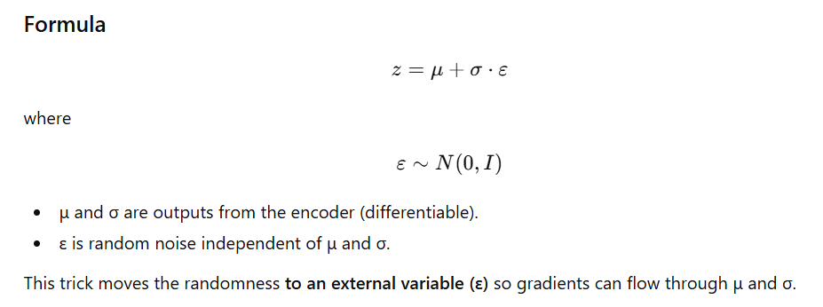
Why Is the Reparameterization Trick Needed?
✔ Enables backpropagation through stochastic nodes
✔ Allows end-to-end training of VAEs
✔ Makes latent space sampling differentiable
✔ Allows optimization of the VAE loss (reconstruction + KL divergence)
Code Example (PyTorch)
class Sampling(torch.nn.Module):
    def forward(self, mu, log_var):
        # Convert log_var to standard deviation
        std = torch.exp(0.5 * log_var)

        # Generate noise ε ~ N(0, 1)
        eps = torch.randn_like(std)

        # Reparameterize: z = μ + σ * ε
        return mu + eps * std
Explanation
log_var→ converted to standard deviation usingexp(0.5 * log_var)eps→ random noise- Output
zis differentiable with respect tomuandstd
Simple Intuition
Instead of sampling z directly from a learned distribution, we sample noise ε (random), and shape it using μ and σ (learned).
This keeps randomness in the model but allows gradients to flow.
91. What Is Deep Reinforcement Learning?
Deep Reinforcement Learning (DRL) combines Reinforcement Learning (RL) with Deep Neural Networks, enabling an agent to learn optimal actions from high-dimensional inputs (such as images, sensor data, or raw pixels).
Key Components
- Agent – Learns and makes decisions.
- Environment – The world with which the agent interacts.
- State (s) – A representation of the current situation.
- Action (a) – Move/decision chosen by the agent.
- Reward (r) – Feedback signal indicating success/failure.
How DRL Works
The agent:
- Observes the current state.
- Takes an action.
- Receives a reward.
- Updates its policy/value function.
- Repeats to maximize long-term reward.
Use Cases
- Game playing (e.g., AlphaGo, Atari, Chess)
- Robotic manipulation
- Autonomous driving
- Real-time resource and energy management
92. How Does Deep Reinforcement Learning Differ from Traditional Reinforcement Learning?
| Feature | Traditional RL | Deep RL |
|---|---|---|
| Function Approximator | Tables, linear models | Deep neural networks |
| Input Representation | Low-dimensional states | High-dimensional inputs (images, pixels) |
| Generalization | Limited to small state spaces | Excellent generalization in large/continuous spaces |
| Exploration Strategy | ε-greedy, softmax | Advanced exploration via policy gradients, entropy regularization |
| Scalability | Not scalable | Highly scalable (GPU-powered) |
| Example | Q-tables for small problems | DQN uses CNNs to learn directly from pixels |
Key Difference
Traditional RL uses Q-tables, while Deep RL uses neural networks to approximate value functions or policies.
93. What Is the Role of Reward Functions in Reinforcement Learning?
The reward function defines what is “good” behavior for the agent. It provides numerical feedback after every action, guiding the agent toward the optimal policy.
Types of Rewards
- Sparse rewards – Rare signals, difficult to learn from.
- Dense rewards – Frequent, informative feedback.
- Shaped rewards – Encourages progress toward the goal.
Design Challenges
- Poor reward design may lead to reward hacking (undesired behavior).
- Sparse rewards can slow down or completely block learning.
- Too much shaping may bias the agent toward suboptimal policies.
Example
For a navigation robot:
- +1 → reaching the target
- –1 → hitting an obstacle
- 0 → normal movement
94. Explain the Concept of Q-Learning
Q-learning is a model-free, off-policy RL algorithm that learns the optimal action-value function:
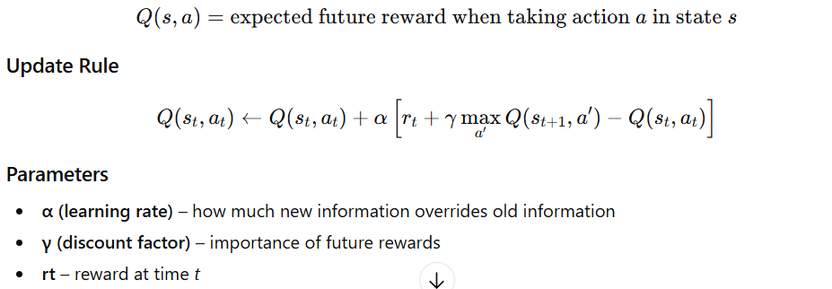
Limitations
- Requires a Q-table, which grows exponentially with states × actions.
- Not suitable for large or continuous environments.
- Cannot handle high-dimensional inputs (images) → solved by DQN (Deep Q-Network).
95. What Is the Purpose of Experience Replay in Deep Reinforcement Learning?
Experience Replay is a technique used in Deep Reinforcement Learning (especially in DQN and its variants) where past experiences
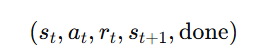
are stored in a buffer and later sampled randomly during training.
Why Use Experience Replay?
Benefits
- Breaks correlation between consecutive experiences (important for stable NN training).
- Stabilizes learning by smoothing out updates.
- Improves sample efficiency by reusing past transitions multiple times.
- Reduces variance and helps the model generalize better.
Implementation Example
import random
from collections import deque

class ReplayBuffer:
    def __init__(self, capacity):
        self.buffer = deque(maxlen=capacity)

    def push(self, state, action, reward, next_state, done):
        self.buffer.append((state, action, reward, next_state, done))

    def sample(self, batch_size):
        return random.sample(self.buffer, batch_size)

# Example usage
buffer = ReplayBuffer(capacity=5)
buffer.push(1, "a", 10, 2, False)
buffer.push(2, "b", 5, 3, False)
buffer.push(3, "c", -1, 4, True)

print("Buffer content:", list(buffer.buffer))
print("Sampled batch:", buffer.sample(2))
Output (Example)
Buffer content: [(1, 'a', 10, 2, False),
                 (2, 'b', 5, 3, False),
                 (3, 'c', -1, 4, True)]

Sampled batch: [(2, 'b', 5, 3, False),
                (1, 'a', 10, 2, False)]
(Note: Sampled batch may vary because of randomness.)
96. What Are Policy Gradient Methods?
Policy Gradient Methods are reinforcement learning techniques that directly optimize the policy function
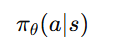
(which outputs a probability distribution over actions) by adjusting its parameters θ to maximize expected return.
Instead of learning value functions (like Q-learning), the algorithm learns the behavior policy itself.
Why Use Policy Gradient Methods?
Advantages
- ✔ Works well with continuous action spaces (robots, control tasks).
- ✔ Stochastic policies → better exploration.
- ✔ Direct policy optimization → avoids large Q-value tables.
- ✔ Suitable for high-dimensional and complex environments.
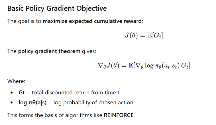
Popular Policy Gradient Algorithms
1. REINFORCE
- Monte-Carlo based policy gradient.
- Updates policy using full episode returns.
- Simple but high variance.
2. Actor–Critic
- Combines:
- Actor → updates policy
- Critic → estimates value function
- Lower variance and more stable.
3. PPO (Proximal Policy Optimization)
- Most widely used modern method.
- Uses clipped objective for stable updates.
- Great performance on robotics & continuous control tasks.
97. How Do Actor-Critic Methods Work in Reinforcement Learning?
Actor–Critic methods combine the strengths of:
- Policy-based learning (Actor) → learns what action to take
- Value-based learning (Critic) → learns how good that action is
This makes training more stable than pure policy gradients and more scalable than Q-learning.
Components
1. Actor
- Represents the policy
- Chooses action
- Learns by ascending the policy gradient
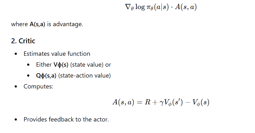
Training Process
- Actor selects an action based on current policy.
- Environment returns reward and next state.
- Critic evaluates: Advantage=TD error\text{Advantage} = \text{TD error}Advantage=TD error
- Actor updates its policy using the critic’s advantage estimate.
- Critic updates its value estimate via TD learning.
This allows low variance, faster convergence, and continuous action space learning.
Code Sketch (PyTorch)
Below is a minimal Actor–Critic example showing action sampling and value evaluation.
import torch
from torch.distributions import Normal

# Actor: outputs mean and std of action distribution
def select_action(state):
    with torch.no_grad():
        mu, sigma = actor(state)        # actor outputs mean, std
        dist = Normal(mu, sigma)
        action = dist.sample()          # sample action
        log_prob = dist.log_prob(action)
    return action, log_prob

# Critic: outputs estimated value or Q-value
def evaluate(state, action):
    value = critic(state, action)       # critic predicts value
    return value
Sample Output (Example Simulation)
State: tensor([0.42, -0.17, 0.89])
Actor Output (mu, sigma): (tensor([0.15]), tensor([0.55]))
Sampled Action: tensor([0.08])
Log Probability: tensor([-1.2563])
Critic Value Estimate: tensor([0.6421])
This shows:
- Actor produced mean=0.15, std=0.55
- Action sampled = 0.08
- Critic estimated value = 0.6421
98. What Is the Role of Exploration vs. Exploitation in Reinforcement Learning?
Reinforcement Learning requires balancing exploration (trying new actions) and exploitation (using known rewarding actions).
✅ Exploration
- Agent tries unfamiliar actions.
- Helps discover better long-term strategies.
- Prevents getting stuck in suboptimal behaviors.
✅ Exploitation
- Uses current knowledge to choose the best-known action.
- Maximizes immediate reward.
Common Exploration Strategies
| Strategy | Description |
|---|---|
| ε-greedy | With probability ε → random action; with (1–ε) → greedy action. |
| Softmax Action Selection | Actions chosen probabilistically based on Q-values. |
| Entropy Regularization | Adds entropy bonus to policy loss → encourages diverse actions in policy gradients. |
Trade-off
- Too much exploitation → Agent gets stuck in local optima.
- Too much exploration → Agent wastes time on poor actions and slows learning.
A good RL agent gradually reduces exploration as it learns.
99. How Does the Proximal Policy Optimization (PPO) Algorithm Work?
Proximal Policy Optimization (PPO) is a state-of-the-art policy gradient algorithm focused on stability, simplicity, and performance.
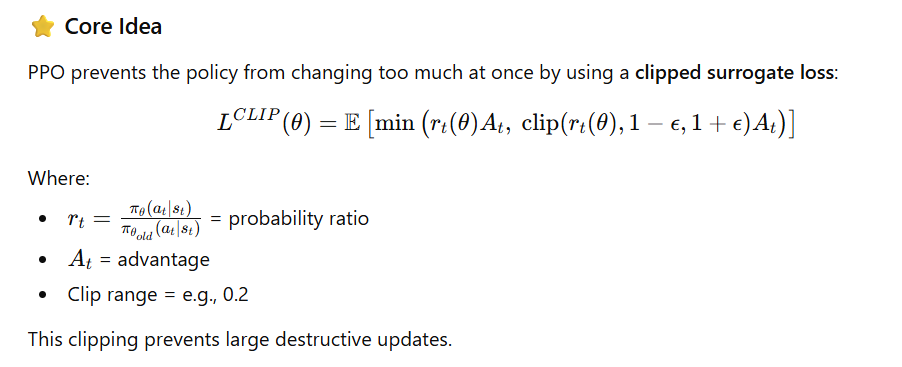
Advantages of PPO
- ✔ Stable training
- ✔ Simple to implement
- ✔ Works well across diverse tasks (robotics, games, control)
- ✔ Less sensitive to hyperparameters than earlier methods
No need for trust-region optimization (like TRPO).
100. What Are the Challenges Associated with Scaling Deep Reinforcement Learning?
Scaling DRL to real-world environments is difficult due to several limitations:
Key Challenges
| Challenge | Description |
|---|---|
| Sample Inefficiency | Requires large amounts of interaction data to learn. |
| Training Instability | Small hyperparameter changes can collapse learning. |
| Sparse Rewards | Hard to learn when environment gives infrequent feedback. |
| High Computational Cost | Needs GPUs/TPUs, parallel environments, large memory. |
| Poor Generalization | Models overfit specific environments; weak transfer learning. |
| Evaluation Difficulty | Stochastic environments make performance hard to measure. |
| Safety & Ethics | Risky or unpredictable behavior in real-world settings. |
Mitigation Strategies
- Curriculum learning
- Imitation or behavior cloning
- Adding intrinsic motivation (curiosity-based RL)
- Auxiliary tasks (multi-task learning)
- Distributed training: Ape-X, IMPALA, V-trace
- Reward shaping or hierarchical RL