Semi-Supervised Learning
What is Semi-Supervised Learning?
Semi-supervised learning is a machine learning approach that uses both labeled and unlabeled data during training. It lies between:
- Supervised learning → requires fully labeled data
- Unsupervised learning → uses no labeled data
The key idea is to leverage a small labeled dataset along with a large unlabeled dataset to improve model accuracy when labeling data is expensive, slow, or difficult.
📌 Why it matters:
In real-world scenarios, unlabeled data is abundant (images, text, logs), while labeled data is costly.
How Semi-Supervised Learning Works
- Data Combination
- Small labeled dataset
- Large unlabeled dataset
- Knowledge Transfer
- Model learns patterns from labeled data
- Applies learned structure to unlabeled data
- Iterative Improvement
- Predicts labels for unlabeled data
- Uses confident predictions to retrain itself
- Consistency Regularization
- Encourages consistent predictions for similar inputs
- Applies to both labeled and unlabeled samples
Types of Semi-Supervised Learning
1. Inductive Methods
- Learn a general model from labeled data
- Apply it to unseen unlabeled data
Examples:
- Self-Training
- Co-Training
2. Transductive Methods
- Focus on labeling a specific unlabeled dataset
- Training and prediction occur together
Examples:
- Label Propagation
- Graph-based learning
3. Generative Models
- Learn the underlying data distribution
- Use both labeled and unlabeled data
Examples:
- Generative Adversarial Networks (GANs)
- Variational Autoencoders (VAEs)
Key Characteristics
- 🔹 Hybrid Approach: Combines supervised and unsupervised ideas
- 🔹 Data Efficient: Works well with limited labeled data
- 🔹 Improved Performance: Better than using labeled data alone
- 🔹 Scalable: Exploits large unlabeled datasets
- 🔹 Flexible: Works for classification, regression, and clustering
Common Semi-Supervised Algorithms
1. Label Propagation
- Builds a similarity graph
- Propagates labels from labeled to unlabeled nodes
Best for: Graph-structured or relational data
2. Self-Training
Steps:
- Train model on labeled data
- Predict labels for unlabeled data
- Select high-confidence predictions
- Add them to training set
- Retrain model
Simple but effective
3. Co-Training
- Uses multiple feature views
- Trains separate classifiers
- Classifiers label data for each other
Works well when features are conditionally independent
4. Generative Models
- Learn joint distribution of features and labels
- Generate synthetic labeled data
Used in: Image generation, NLP, speech processing
5. Graph-Based Methods
- Data points = nodes
- Similarity = edges
- Labels spread through graph structure
Real-World Applications
- 📧 Spam Detection: Few labeled emails, many unlabeled
- 🏥 Medical Diagnosis: Limited expert-labeled data
- 🖼️ Image Classification: Small labeled image sets
- 🗣️ Speech Recognition: Large unlabeled audio corpora
- 🌐 Web Page Classification: Minimal manual labeling
Advantages
- ✔ Reduces labeling cost
- ✔ Improves model accuracy
- ✔ Uses abundant unlabeled data
- ✔ Effective in real-world scenarios
Disadvantages
- ❌ Error propagation risk
- ❌ Assumes labeled and unlabeled data share structure
- ❌ Sensitive to initial labeled data quality
- ❌ More complex than supervised learning
One-Line Exam Definition 📌
Semi-supervised learning uses a small amount of labeled data along with a large amount of unlabeled data to improve learning accuracy and efficiency.
Comparison Summary
| Learning Type | Labeled Data | Unlabeled Data |
|---|---|---|
| Supervised | Yes | No |
| Unsupervised | No | Yes |
| Semi-Supervised | Limited | Yes |
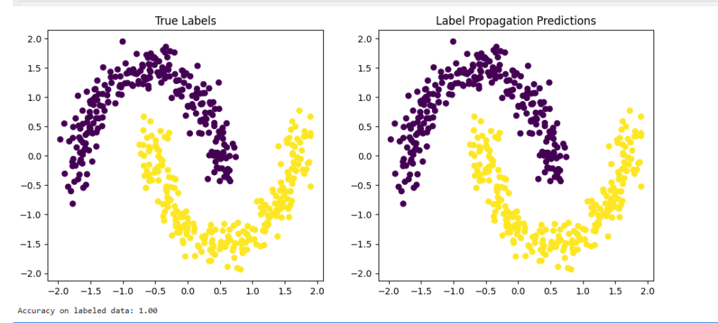
Example 1: Label Propagation (Semi-Supervised Classification)
✔ Uses graph-based learning
✔ Very effective when data has clear structure
import numpy as np
import matplotlib.pyplot as plt
from sklearn.datasets import make_moons
from sklearn.semi_supervised import LabelPropagation
from sklearn.model_selection import train_test_split
from sklearn.preprocessing import StandardScaler

# Generate dataset
X, y = make_moons(n_samples=500, noise=0.1, random_state=42)

# Scale features
X = StandardScaler().fit_transform(X)

# Keep only 20% labeled
X_labeled, X_unlabeled, y_labeled, y_unlabeled = train_test_split(
    X, y, test_size=0.8, stratify=y, random_state=42
)

# Unlabeled data gets label -1
X_combined = np.vstack((X_labeled, X_unlabeled))
y_combined = np.hstack((y_labeled, -np.ones(len(y_unlabeled))))

# Train Label Propagation
model = LabelPropagation(kernel="rbf", gamma=20)
model.fit(X_combined, y_combined)

# Predict all labels
predictions = model.predict(X)

# Visualization
plt.figure(figsize=(12, 5))

plt.subplot(1, 2, 1)
plt.scatter(X[:, 0], X[:, 1], c=y, cmap="viridis")
plt.title("True Labels")

plt.subplot(1, 2, 2)
plt.scatter(X[:, 0], X[:, 1], c=predictions, cmap="viridis")
plt.title("Label Propagation Predictions")

plt.show()

print(f"Accuracy on labeled data: {model.score(X_labeled, y_labeled):.2f}")
📌 Key idea: Labels spread through a similarity graph.
Example 2: Self-Training with Logistic Regression
✔ Simple and widely used
✔ Risk: error propagation if confidence is wrong
import numpy as np
from sklearn.datasets import load_digits
from sklearn.linear_model import LogisticRegression
from sklearn.model_selection import train_test_split

# Load dataset
X, y = load_digits(return_X_y=True)

# Only 30% labeled
X_labeled, X_unlabeled, y_labeled, _ = train_test_split(
    X, y, test_size=0.7, stratify=y, random_state=42
)

model = LogisticRegression(max_iter=1000)

for iteration in range(5):
    model.fit(X_labeled, y_labeled)

    probs = model.predict_proba(X_unlabeled)
    confidence = probs.max(axis=1)
    predictions = probs.argmax(axis=1)

    # Select top 20% confident predictions
    threshold = np.percentile(confidence, 80)
    mask = confidence >= threshold

    X_labeled = np.vstack((X_labeled, X_unlabeled[mask]))
    y_labeled = np.hstack((y_labeled, predictions[mask]))
    X_unlabeled = X_unlabeled[~mask]

    print(f"Iteration {iteration+1}: Added {mask.sum()} samples")

print(f"Final accuracy on labeled data: {model.score(X_labeled, y_labeled):.2f}")
📌 Use when: You trust your model’s confidence estimates.
Iteration 1: Added 252 samples
Iteration 2: Added 202 samples
Iteration 3: Added 161 samples
Iteration 4: Added 129 samples
Iteration 5: Added 103 samples
Final accuracy on labeled data: 1.00
Example 3: Co-Training (Two Independent Views)
✔ Works best when features are conditionally independent
✔ Common in text + metadata problems
⚠️ Important Fix
Your original version removed y_unlabeled twice → bug
Below is the correct and safe version.
import numpy as np
from sklearn.datasets import make_classification
from sklearn.naive_bayes import GaussianNB
from sklearn.linear_model import LogisticRegression
from sklearn.model_selection import train_test_split

# Generate dataset
X, y = make_classification(
    n_samples=1000, n_features=20, n_informative=10,
    n_redundant=5, random_state=42
)

# Two views
X_view1, X_view2 = X[:, :10], X[:, 10:]

# Only 20% labeled
X_labeled, X_unlabeled, y_labeled, _ = train_test_split(
    X, y, test_size=0.8, stratify=y, random_state=42
)

X1_labeled, X2_labeled = X_labeled[:, :10], X_labeled[:, 10:]
X1_unlabeled, X2_unlabeled = X_unlabeled[:, :10], X_unlabeled[:, 10:]

clf1 = GaussianNB()
clf2 = LogisticRegression(max_iter=1000)

for iteration in range(10):
    clf1.fit(X1_labeled, y_labeled)
    clf2.fit(X2_labeled, y_labeled)

    probs1 = clf1.predict_proba(X1_unlabeled)
    probs2 = clf2.predict_proba(X2_unlabeled)

    conf1 = probs1.max(axis=1)
    conf2 = probs2.max(axis=1)

    mask1 = conf1 >= 0.9
    mask2 = conf2 >= 0.9

    X1_labeled = np.vstack((X1_labeled, X1_unlabeled[mask1]))
    X2_labeled = np.vstack((X2_labeled, X2_unlabeled[mask2]))
    y_labeled = np.hstack((y_labeled,
                           probs1.argmax(axis=1)[mask1],
                           probs2.argmax(axis=1)[mask2]))

    combined_mask = mask1 | mask2
    X1_unlabeled = X1_unlabeled[~combined_mask]
    X2_unlabeled = X2_unlabeled[~combined_mask]

    print(f"Iteration {iteration+1}: Added {combined_mask.sum()} samples")

print(f"Final accuracy (View 1): {clf1.score(X1_labeled, y_labeled):.2f}")
print(f"Final accuracy (View 2): {clf2.score(X2_labeled, y_labeled):.2f}")
✅ Example 4: Semi-Supervised Learning with Generative Models
- Use Autoencoder → train on all data
- Use Classifier → train only on labeled data
- Encoder learns representation from unlabeled data
- Classifier benefits from that representation
✔ Corrected & Safe Code
import numpy as np
import tensorflow as tf
from tensorflow import keras
from sklearn.datasets import make_moons
from sklearn.model_selection import train_test_split
from sklearn.preprocessing import StandardScaler
from sklearn.metrics import accuracy_score

# Generate data
X, y = make_moons(n_samples=1000, noise=0.1, random_state=42)
X = StandardScaler().fit_transform(X)

# Only 10% labeled
X_labeled, X_unlabeled, y_labeled, _ = train_test_split(
    X, y, test_size=0.9, stratify=y, random_state=42
)

input_dim = X.shape[1]
latent_dim = 2

# Encoder
encoder = keras.Sequential([
    keras.layers.Dense(32, activation="relu", input_shape=(input_dim,)),
    keras.layers.Dense(16, activation="relu"),
    keras.layers.Dense(latent_dim)
])

# Decoder
decoder = keras.Sequential([
    keras.layers.Dense(16, activation="relu", input_shape=(latent_dim,)),
    keras.layers.Dense(32, activation="relu"),
    keras.layers.Dense(input_dim)
])

# Autoencoder
autoencoder_input = keras.Input(shape=(input_dim,))
encoded = encoder(autoencoder_input)
decoded = decoder(encoded)
autoencoder = keras.Model(autoencoder_input, decoded)

autoencoder.compile(
    optimizer="adam",
    loss="mse"
)

# Train autoencoder on ALL data
autoencoder.fit(
    X, X,
    epochs=50,
    batch_size=32,
    validation_split=0.1,
    verbose=0
)

# Classifier on top of encoder
classifier = keras.Sequential([
    keras.layers.Dense(16, activation="relu", input_shape=(latent_dim,)),
    keras.layers.Dense(1, activation="sigmoid")
])

classifier.compile(
    optimizer="adam",
    loss="binary_crossentropy",
    metrics=["accuracy"]
)

# Train classifier ONLY on labeled data
classifier.fit(
    encoder.predict(X_labeled),
    y_labeled,
    epochs=50,
    batch_size=16,
    verbose=0
)

# Evaluate
y_pred = (classifier.predict(encoder.predict(X_labeled)) > 0.5).astype(int)
accuracy = accuracy_score(y_labeled, y_pred)

print(f"Classifier accuracy on labeled data: {accuracy:.2f}")
4/4 ━━━━━━━━━━━━━━━━━━━━ 0s 28ms/step
4/4 ━━━━━━━━━━━━━━━━━━━━ 0s 9ms/step
4/4 ━━━━━━━━━━━━━━━━━━━━ 0s 22ms/step
Classifier accuracy on labeled data: 0.87
✅ Example 5: Graph-Based Semi-Supervised Learning (Label Spreading)
✔ Your original logic was mostly correct
✔ Minor cleanup and explanation below
✔ Clean & Final Version
import numpy as np
import matplotlib.pyplot as plt
from sklearn.datasets import make_circles
from sklearn.semi_supervised import LabelSpreading
from sklearn.model_selection import train_test_split

# Generate circular data
X, y = make_circles(n_samples=500, noise=0.1, factor=0.5, random_state=42)

# Only 15% labeled
X_labeled, X_unlabeled, y_labeled, y_unlabeled = train_test_split(
    X, y, test_size=0.85, stratify=y, random_state=42
)

# Combine data
X_combined = np.vstack((X_labeled, X_unlabeled))
y_combined = np.hstack((y_labeled, -np.ones(len(y_unlabeled))))

# Train Label Spreading model
model = LabelSpreading(kernel="rbf", gamma=15, max_iter=1000)
model.fit(X_combined, y_combined)

# Predict
predictions = model.predict(X)

# Visualization
plt.figure(figsize=(12, 5))

plt.subplot(1, 2, 1)
plt.scatter(X[:, 0], X[:, 1], c=y, cmap="viridis")
plt.title("True Labels")

plt.subplot(1, 2, 2)
plt.scatter(X[:, 0], X[:, 1], c=predictions, cmap="viridis")
plt.title("Label Spreading Predictions")

plt.show()

print(f"Accuracy on labeled data: {model.score(X_labeled, y_labeled):.2f}")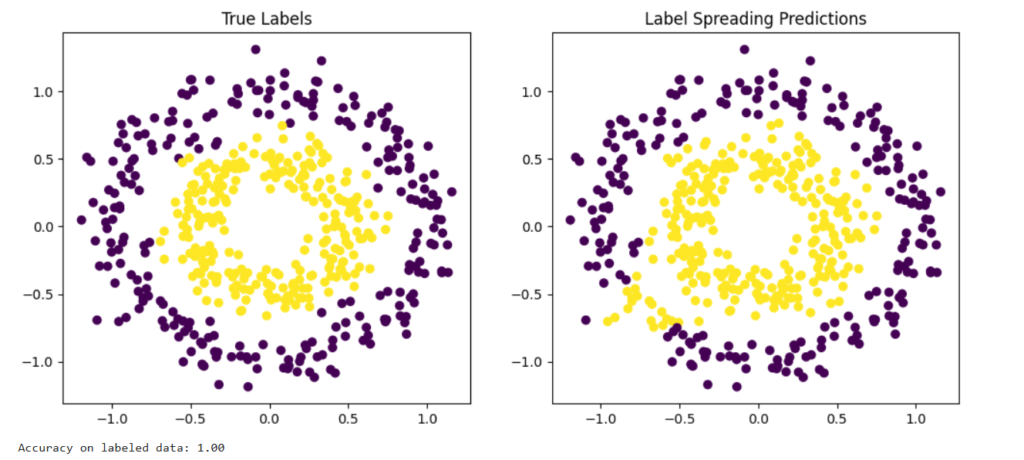
Semi-Supervised Learning – Real-World Examples
1. Medical Image Analysis
Input:
- Medical images (X-rays, MRIs, CT scans) with limited expert annotations
Output:
- Disease diagnosis or anomaly detection
Algorithms:
- Self-Training
- Co-Training (multi-view learning)
Use Cases:
- Tumor detection
- Early disease diagnosis with limited labeled data
2. Web Page Classification
Input:
- Millions of web pages with very few manually labeled samples
Output:
- Web page categories (news, shopping, education, entertainment)
Algorithms:
- Label Propagation
- Graph-Based Semi-Supervised Methods
Use Cases:
- Web content organization
- Search engine indexing
3. Speech Recognition
Input:
- Audio recordings with limited transcriptions
Output:
- Text transcriptions
Algorithms:
- Generative Models
- Self-Training
Use Cases:
- Voice assistants
- Low-resource language speech recognition
4. Financial Fraud Detection
Input:
- Transaction data with very few labeled fraud cases
Output:
- Fraudulent vs legitimate transactions
Algorithms:
- Semi-Supervised Anomaly Detection
- Graph-Based Methods
Use Cases:
- Credit card fraud detection
- Banking security systems
5. Recommendation Systems
Input:
- User–item interaction data with limited explicit ratings
Output:
- Personalized recommendations
Algorithms:
- Graph-Based Learning
- Co-Training
Use Cases:
- Netflix movie recommendations
- Amazon product suggestions
Advantages of Semi-Supervised Learning
- ✔ Data Efficient: Uses large amounts of unlabeled data effectively
- ✔ Cost-Effective: Reduces expensive manual labeling
- ✔ Improved Accuracy: Often outperforms purely supervised models
- ✔ Scalable: Suitable for very large datasets
- ✔ Flexible: Works across text, images, audio, and graphs
Disadvantages of Semi-Supervised Learning
- ❌ High Complexity: More difficult to design and implement
- ❌ Algorithm Selection: Choosing the right method is non-trivial
- ❌ Evaluation Challenges: Lack of ground truth complicates validation
- ❌ Convergence Issues: Some methods may diverge or propagate errors
- ❌ Hyperparameter Sensitivity: Performance depends heavily on tuning
Best Practices for Semi-Supervised Learning
- High-Quality Labeled Data: Ensure labeled samples are accurate and representative
- Algorithm Selection: Match the method to data type and problem structure
- Hyperparameter Tuning: Carefully tune thresholds, confidence levels, and graph parameters
- Evaluation Strategy: Use cross-validation on labeled data and monitor consistency
- Iterative Refinement: Gradually improve the model through multiple iterations
- Domain Knowledge: Incorporate expert knowledge to guide model decisions
📌 One-Line Exam / Interview Summary
Semi-supervised learning combines a small amount of labeled data with large unlabeled datasets to improve learning efficiency, accuracy, and scalability.