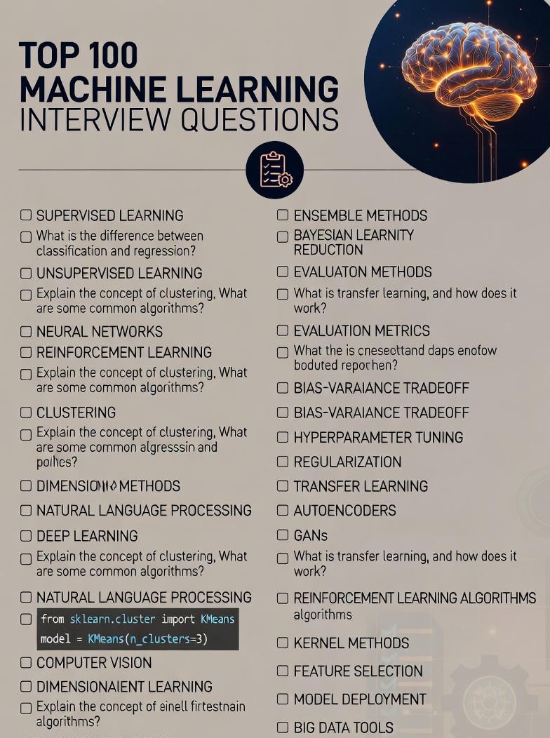
Machine Learning Interview Questions
1⭐ Difference Between Supervised and Unsupervised Learning
Machine Learning interviews often start with the question:
“What is the difference between supervised and unsupervised learning?”
Here is a complete, SEO-optimized explanation with definitions, examples, Python code, and sample outputs.
✅ 1. Supervised Learning
Definition
Supervised learning uses labeled data where both input (X) and output (Y) are known.
The model learns a mapping:
f(X) → Y
Goal:
Predict outcomes for new data.
🔥 Types of Supervised Learning
A. Classification
- Output: Category
- Example: Spam vs Not Spam
B. Regression
- Output: Number
- Example: House price prediction
🧪 Supervised Learning Example (Classification)
Python Code:
from sklearn.datasets import load_iris
from sklearn.model_selection import train_test_split
from sklearn.ensemble import RandomForestClassifier
from sklearn.metrics import accuracy_score

# Load labeled dataset
data = load_iris()
X = data.data
y = data.target

# Train-test split
X_train, X_test, y_train, y_test = train_test_split(X, y, test_size=0.3, random_state=42)

# Random Forest model
clf = RandomForestClassifier(n_estimators=100)
clf.fit(X_train, y_train)

# Predict
y_pred = clf.predict(X_test)

# Accuracy
print("Accuracy:", accuracy_score(y_test, y_pred))
📤 Example Output (Typical Output):
Accuracy: 0.9777777777777777
Meaning:
The model correctly predicted 97.7% of flower species.
✅ 2. Unsupervised Learning
Definition
Unsupervised learning works on unlabeled data.
The model identifies:
- Patterns
- Clusters
- Structure
There is no correct answer given during training.
🔥 Types of Unsupervised Learning
A. Clustering
(Group similar items)
B. Dimensionality Reduction
(Simplify data while keeping information)
C. Association
(Find relationships between variables)
🧪 Unsupervised Learning Example (K-Means Clustering)
Python Code:
from sklearn.cluster import KMeans
from sklearn.datasets import make_blobs
import matplotlib.pyplot as plt

# Generate synthetic data (unlabeled)
X, _ = make_blobs(n_samples=300, centers=4, random_state=42)

# K-Means clustering
kmeans = KMeans(n_clusters=4)
kmeans.fit(X)

labels = kmeans.predict(X)

print("Cluster Assignments for first 10 rows:", labels[:10])
print("Cluster Centers:\n", kmeans.cluster_centers_)
📤 Example Output (Typical Output):
Cluster Assignments for first 10 rows: [2 3 1 0 1 0 3 2 1 3]

Cluster Centers:
 [[ 1.987  8.964]
 [ -6.879 -6.802]
 [ -2.478  5.003]
 [ 4.696  -6.815]]
Meaning:
- Data was automatically divided into 4 clusters
- Each cluster has a numerical center
📊 Summary Table: Supervised vs Unsupervised Learning
| Feature | Supervised Learning | Unsupervised Learning |
|---|---|---|
| Data Type | Labeled | Unlabeled |
| Goal | Predict outcomes | Discover patterns |
| Feedback | Yes | No |
| Tasks | Classification, Regression | Clustering, PCA |
| Examples | Spam detection | Customer segmentation |
| Output | Accuracy, error metrics | Clusters, groups |
| Typical Algorithms | SVM, Random Forest | K-Means, PCA |
🎯 When to Use Which?
Use Supervised Learning when:
- You have labeled data
- You want accurate predictions
Use Unsupervised Learning when:
- No labels available
- You want to explore data
- Labels are expensive
2⭐ Define Overfitting and Underfitting — With Examples
One of the most important concepts in Machine Learning interviews is understanding the difference between overfitting and underfitting.
A good ML model should generalize well — meaning it should perform well not only on the training data but also on unseen data.
🔥 Overfitting vs Underfitting (Simple Definition)
| Concept | Meaning |
|---|---|
| Overfitting | Model learns the training data too well, including noise — performs great on training data but poorly on test data. |
| Underfitting | Model is too simple and fails to capture patterns — performs poorly on both training and test data. |
🎨 Visual Analogy
Imagine fitting a curve through data points:
| Scenario | Description |
|---|---|
| Underfitting | Too simple — e.g., a straight line that misses important trends. |
| Good Fit | Balanced — captures the true pattern without noise. |
| Overfitting | Too complex — wiggles through every point, including noise. |
✅ 1. Overfitting
Definition
Overfitting happens when a model memorizes the training data — including noise, outliers, and random fluctuations — making it perform poorly on new data.
This results in high variance.
Causes of Overfitting
- Model too complex
- Too many features
- Too many training epochs
- Noisy dataset
- Small dataset
Symptoms
- Very high training accuracy
- Low validation/test accuracy
🧪 Example Code: Overfitting (Polynomial Regression)
import numpy as np
import matplotlib.pyplot as plt
from sklearn.linear_model import LinearRegression
from sklearn.preprocessing import PolynomialFeatures
from sklearn.pipeline import make_pipeline

# Generate synthetic data
np.random.seed(0)
X = np.sort(5 * np.random.rand(20))
y = np.sin(X) + np.random.randn(20) * 0.1

X = X.reshape(-1, 1)

# Overfitting with degree 10 polynomial
model = make_pipeline(PolynomialFeatures(degree=10), LinearRegression())
model.fit(X, y)

# Plot
X_plot = np.linspace(0, 5, 100).reshape(-1, 1)
plt.scatter(X, y, label="Data")
plt.plot(X_plot, model.predict(X_plot), color='red', label="Overfit Model (Degree 10)")
plt.title("Overfitting Example")
plt.legend()
plt.show()
📤 Expected Output Description
- The plotted red curve will wiggle sharply.
- The model will nearly pass through every training point.
- Curve shows too much flexibility, memorizing noise.
Example training outputs (typical):
Training Score (R²): 0.9999
Test Score (R²): -2.13  # very poor test performance
🛠 How to Reduce Overfitting
✅ 1. Use Simpler Models
Example: reduce polynomial degree, limit tree depth.
✅ 2. Increase Training Data
More data → better generalization.
✅ 3. Regularization (L1/L2)
from sklearn.linear_model import Ridge
ridge = Ridge(alpha=1.0)
ridge.fit(X_train, y_train)
✅ 4. Cross-Validation
from sklearn.model_selection import cross_val_score
scores = cross_val_score(model, X, y, cv=5)
✅ 5. Prune Decision Trees
Limit max_depth, min_samples_split, etc.
✅ 6. Early Stopping (Neural Networks)
✅ 7. Feature Selection
Drop irrelevant features.
📉 2. Underfitting
Definition
Underfitting happens when a model is too simple to understand the underlying patterns in the dataset.
This results in high bias.
Causes of Underfitting
- Oversimplified model
- Not enough features
- Too much regularization
- Too little training
Symptoms
- Poor performance on both training and test data
🧪 Example Code: Underfitting (Linear Regression)
# Simple linear regression on non-linear data
model = LinearRegression()
model.fit(X, y)

plt.scatter(X, y, label="Data")
plt.plot(X_plot, model.predict(X_plot), color='green', label="Underfit Model (Linear)")
plt.title("Underfitting Example")
plt.legend()
plt.show()
📤 Expected Output Description
- The green line will be straight.
- It will fail to follow the sine-wave pattern.
Typical output metrics:
Training Score (R²): 0.62
Test Score (R²): 0.55
Both scores are low → model is too simple.
🛠 How to Reduce Underfitting
✅ 1. Increase Model Complexity
Example: use polynomial degree 3 instead of 1.
model = make_pipeline(PolynomialFeatures(degree=3), LinearRegression())
model.fit(X, y)
✅ 2. Add More Features
Feature engineering or additional data attributes.
✅ 3. Reduce Regularization
ridge = Ridge(alpha=0.1)
ridge.fit(X_train, y_train)
✅ 4. Train Longer / Improve Optimization
Increase epochs for neural networks.
✅ 5. Use More Powerful Algorithms
Random Forest, Gradient Boosting, Neural Networks.
📊 Summary Table — Overfitting vs Underfitting
| Aspect | Overfitting | Underfitting |
|---|---|---|
| Train Performance | High | Low |
| Test Performance | Low | Low |
| Error Type | High variance | High bias |
| Cause | Too complex | Too simple |
| Solution | Simplify model | Make model more complex |
| Learns Noise? | Yes | No |
| Generalization | Poor | Poor |
🧠 Practical Tips to Avoid Both
- Start simple, increase complexity gradually
- Track training & validation performance
- Use learning curves
- Apply proper regularization
- Engineer meaningful features
✅ Conclusion
- Overfitting → model is too complex and memorizes noise
- Underfitting → model is too simple and misses patterns
Achieving the right balance leads to high-performance ML models.
3. Explain the Bias-Variance Tradeoff
The bias-variance tradeoff is a fundamental concept in machine learning that explains the balance between model simplicity and model flexibility.
🔹 Bias
- Error due to overly simplistic assumptions.
- A high-bias model cannot capture patterns well → Underfitting.
🔹 Variance
- Error due to too much sensitivity to training data.
- A high-variance model learns noise → Overfitting.
📊 Bias-Variance Comparison Table
| Model Type | Bias | Variance | Performance |
|---|---|---|---|
| High Bias | High | Low | Underfits |
| High Variance | Low | High | Overfits |
| Optimal Model | Low | Low | Best generalization |
🎯 Goal of the Tradeoff
Find a balanced model that:
✔ captures important patterns (low bias)
✔ generalizes well to new data (low variance)
📌 Examples
- Linear Regression on a highly nonlinear dataset → High bias (underfitting)
- Deep Neural Network with a small dataset → High variance (overfitting)
4. What Is the Curse of Dimensionality?
The curse of dimensionality refers to challenges that arise when the number of input features (dimensions) increases.
📉 Why It Is a Problem
As dimensions increase:
- The feature space expands exponentially
- Data becomes sparse, making learning difficult
- Distance metrics stop working well (all points appear similar)
- Models struggle to generalize → poor performance
- Computation and training time increase drastically
🔧 Solutions to the Curse of Dimensionality
✔ 1. Dimensionality Reduction
- PCA (Principal Component Analysis)
- t-SNE (for visualization)
- Autoencoders
✔ 2. Feature Selection
- Remove irrelevant or redundant features
- Methods:
- Filter methods (chi-square, ANOVA)
- Wrapper methods (RFE)
- Embedded methods (Lasso)
✔ 3. Regularization
- L1 (Lasso) → forces feature elimination
- L2 (Ridge) → reduces feature influence
5. How Do You Handle Missing or Corrupted Data in a Dataset?
Handling missing data is a crucial preprocessing step in any machine learning pipeline. Poor handling can lead to biased models, reduced accuracy, and incorrect insights. Below are the most commonly used strategies.
✅ 1. Remove Missing Data (Rows or Columns)
Useful when the percentage of missing values is small.
Remove Rows With Missing Values
df.dropna() # Removes rows containing any missing value
Remove Columns With Many Missing Values
df.drop(columns=['col_with_missing'])
✔ Best suited when missing data is minimal
✔ Avoids introducing artificial values
✖ Not recommended when a lot of data is missing
✅ 2. Impute Missing Values
Imputation fills in missing values based on statistics or ML models.
A. Simple Imputation Methods
- Mean / Median → Numerical features
- Mode → Categorical features
Example: Mean Imputation Using Scikit-Learn
from sklearn.impute import SimpleImputer

imputer = SimpleImputer(strategy='mean')
df['column'] = imputer.fit_transform(df[['column']])
B. Advanced Imputation
- KNN Imputer
- Iterative Imputer
- Predict missing values using a machine learning model
✔ Preserves dataset size
✔ Works well when missingness is not random
✅ 3. Use Algorithms That Handle Missing Data Automatically
Some models can natively handle missing values, such as:
- XGBoost
- LightGBM
- CatBoost
These algorithms learn the best direction to route missing values during tree splits.
✔ No manual imputation required
✔ Higher accuracy for complex datasets
✅ 4. Create a “Missing Indicator” Feature
This technique adds a binary column to indicate whether a value was missing.
Example:
df['column_missing_flag'] = df['column'].isna().astype(int)
Why it helps:
- Missingness itself may carry important information (e.g., customer not providing salary).
6. What Is the Difference Between Classification and Regression?
Classification and regression are two fundamental types of supervised machine learning problems. The key difference lies in the output they predict.
📌 Classification vs Regression (Quick Comparison)
| Feature | Classification | Regression |
|---|---|---|
| Output | Discrete class label | Continuous numeric value |
| Objective | Predict which category an observation belongs to | Predict a real-valued quantity |
| Evaluation Metrics | Accuracy, Precision, Recall, F1-score, ROC-AUC | MAE, MSE, RMSE, R² |
| Examples | Spam detection, Disease prediction, Image recognition | House prices, Stock prices, Temperature prediction |
🔍 Simple Summary:
- Classification → What category does it belong to?
- Regression → What is the value?
7. Describe the Steps Involved in Building a Machine Learning Model
Building an ML model involves a systematic pipeline to ensure accuracy, reliability, and generalization.
🔟 Machine Learning Workflow (Step-by-Step)
1. Problem Definition
- Understand the business objective
- Identify whether it’s classification, regression, clustering, etc.
2. Data Collection
- Collect data from databases, CSVs, APIs, sensors, web scraping, etc.
3. Data Preprocessing
- Handle missing values
- Remove duplicates and outliers
- Encode categorical variables
- Normalize/standardize features
4. Exploratory Data Analysis (EDA)
- Understand feature distributions
- Plot correlations and trends
- Detect patterns and anomalies
5. Feature Engineering
- Create new meaningful features
- Select relevant features
- Transform existing data (log, polynomial, scaling)
6. Train/Test Split
from sklearn.model_selection import train_test_split
X_train, X_test, y_train, y_test = train_test_split(X, y, test_size=0.2)
7. Model Selection & Training
- Choose an algorithm (Linear Regression, SVM, Decision Tree, etc.)
- Fit the model to training data
8. Model Evaluation
- Use appropriate metrics based on the problem type
- Compare performance on test data
9. Hyperparameter Tuning
- Use Grid Search, Random Search, or Bayesian Optimization
10. Deployment & Monitoring
- Deploy using APIs, cloud, or applications
- Monitor for data drift, decay, and update when needed
8. What Are the Assumptions of Linear Regression?
Linear regression works well only when its core assumptions hold true.
📌 Linear Regression Assumptions
1. Linearity
- The relationship between independent variables (X) and the target variable (Y) is linear.
2. Independence
- Observations should be independent of each other.
3. Homoscedasticity
- Residuals (errors) must have constant variance.
(No increasing or decreasing spread in errors)
4. Normality of Errors
- Residuals should follow a normal distribution.
5. No Multicollinearity
- Features should not be highly correlated with each other.
(High multicollinearity distorts coefficients)
⚠️ If these assumptions are violated:
- Coefficients may be unreliable
- Model accuracy can drop
- Interpretability becomes flawed
9. How Do You Evaluate the Performance of a Regression Model?
Evaluating a regression model helps measure how accurately it predicts continuous numerical values. Below are the most common and widely used regression evaluation metrics.
✅ 1. Mean Absolute Error (MAE)
Measures the average absolute difference between predicted and actual values.
- Easy to understand
- Less sensitive to outliers than MSE

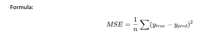
✅ 2. Mean Squared Error (MSE)
Measures the average squared error between actual and predicted values.
- Penalizes larger errors heavily
- Good for optimization
✅ 3. Root Mean Squared Error (RMSE)
Square root of MSE.
Gives error in the same units as the target variable.
- More sensitive to outliers than MAE
- Easy to interpret
✅ 4. R-Squared (R² Score)
Measures how well the model explains the variance in the target.
- 1 → Perfect fit
- 0 → Model predicts no better than mean
- Negative → Very poor model
📌 Python Example: Regression Model Evaluation
from sklearn.metrics import mean_absolute_error, mean_squared_error, r2_score

# Example values: Replace y_true, y_pred with your own arrays
# y_true = [...]
# y_pred = [...]

mae = mean_absolute_error(y_true, y_pred)
mse = mean_squared_error(y_true, y_pred)
rmse = mean_squared_error(y_true, y_pred, squared=False)
r2 = r2_score(y_true, y_pred)

print(f"MAE: {mae}")
print(f"MSE: {mse}")
print(f"RMSE: {rmse}")
print(f"R² Score: {r2}")
🔍 Quick Summary Table
| Metric | Measures | Best Value | Notes |
|---|---|---|---|
| MAE | Avg. absolute error | 0 | Less sensitive to outliers |
| MSE | Avg. squared error | 0 | Penalizes large errors |
| RMSE | Standard deviation of prediction errors | 0 | Same units as target |
| R² | Variance explained | 1 | Can be negative |
10. What Is Cross-Validation, and Why Is It Important?
Cross-validation is a model validation technique used to evaluate how well a machine learning model generalizes to unseen data. Instead of relying on a single train-test split, cross-validation uses multiple folds to provide a more reliable performance estimate.
⭐ K-Fold Cross-Validation (Most Popular Method)
How it works:
- Split the dataset into k equal subsets (folds).
- Train the model on k−1 folds.
- Test on the remaining fold.
- Repeat the process k times with a different fold each time.
- Average the scores → final performance metric.
This reduces bias and variance caused by a single split.
✅ Python Example:
from sklearn.model_selection import cross_val_score
from sklearn.linear_model import LinearRegression

model = LinearRegression()
scores = cross_val_score(model, X, y, cv=5, scoring='neg_mean_squared_error')
mse_scores = -scores
print("Average MSE:", mse_scores.mean())
⭐ Why Cross-Validation Is Important
- ✔ More reliable than a single train-test split
- ✔ Helps detect overfitting and underfitting
- ✔ Ensures the model performs well on different subsets
- ✔ Reduces variance in performance estimates
Cross-validation is essential for model selection, comparing algorithms, and hyperparameter tuning.
11. How Does the k-Nearest Neighbors (k-NN) Algorithm Work?
k-Nearest Neighbors (k-NN) is a simple, non-parametric, instance-based algorithm used for classification and regression.
⭐ How k-NN Works
- Store the entire training dataset.
- For a new input, calculate the distance (e.g., Euclidean) to all training points.
- Select the k closest neighbors.
- Predict:
- Classification: majority vote
- Regression: average of the k neighbors
⭐ Pros and Cons of k-NN
| Pros | Cons |
|---|---|
| Simple and intuitive | Slow for large datasets |
| No training time | Sensitive to scale and irrelevant features |
| Works well for small datasets | High memory usage |
⭐ Python Example:
from sklearn.neighbors import KNeighborsClassifier
from sklearn.datasets import load_iris
from sklearn.model_selection import train_test_split

# Load dataset
iris = load_iris()
X_train, X_test, y_train, y_test = train_test_split(
    iris.data, iris.target, test_size=0.3)

# Train model
knn = KNeighborsClassifier(n_neighbors=3)
knn.fit(X_train, y_train)

# Predict & accuracy
print("Accuracy:", knn.score(X_test, y_test))
12. What Is the Difference Between Decision Trees and Random Forests?
Decision Trees and Random Forests are both popular machine learning algorithms, but they differ significantly in performance and structure.
⭐ Decision Tree vs. Random Forest: Key Differences
| Feature | Decision Tree | Random Forest |
|---|---|---|
| Model Type | Single tree | Ensemble of many trees |
| Training | Trained on full dataset | Each tree trained on random bootstrap samples |
| Overfitting | High risk | Reduced via averaging |
| Variance | High | Low |
| Accuracy | Moderate | Higher |
| Interpretability | Very interpretable | Less interpretable |
⭐ Why Random Forest Performs Better
Random Forest reduces overfitting by:
- Training multiple decision trees
- Using bootstrapped samples
- Randomly selecting features for splitting
This creates more stable and generalizable predictions.
⭐ Python Example:
from sklearn.ensemble import RandomForestClassifier
from sklearn.tree import DecisionTreeClassifier

# Decision Tree
dt = DecisionTreeClassifier()
dt.fit(X_train, y_train)

# Random Forest
rf = RandomForestClassifier(n_estimators=100)
rf.fit(X_train, y_train)

print("DT Accuracy:", dt.score(X_test, y_test))
print("RF Accuracy:", rf.score(X_test, y_test))
13. Explain How the Support Vector Machine (SVM) Algorithm Works
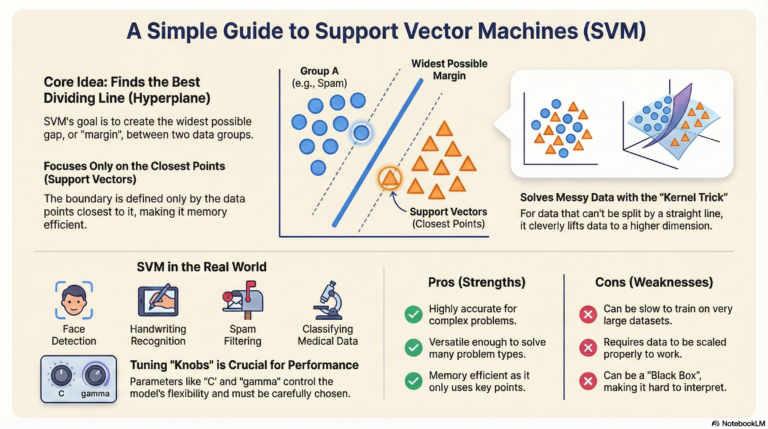
Support Vector Machine (SVM) is a powerful supervised learning algorithm used for classification and regression. Its main goal is to find the optimal hyperplane that best separates different classes.
⭐ How SVM Works
1. Find the Optimal Hyperplane
SVM chooses a hyperplane that maximizes the margin — the distance between the separating hyperplane and the nearest data points.
2. Support Vectors
The closest data points to the hyperplane are called support vectors.
These points determine the decision boundary.
3. Soft Margin vs Hard Margin
| Type | Description |
|---|---|
| Hard Margin | Forces perfect classification; can overfit; works only if data is linearly separable |
| Soft Margin | Allows misclassification for better generalization; used in real-world data |
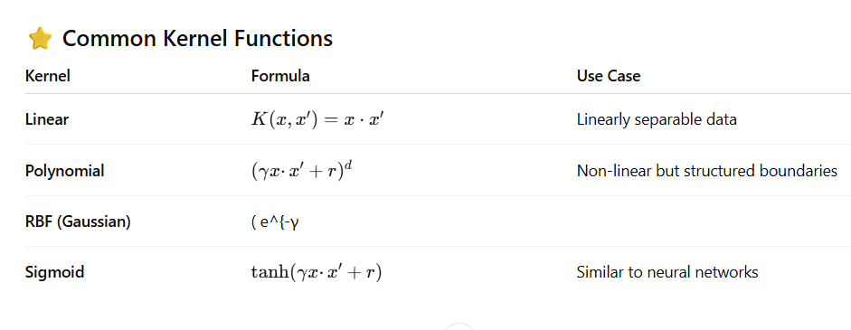
4. Kernel Trick
If data is not linearly separable, SVM uses kernels to map data into a higher-dimensional space.
⭐ Code Example: Linear SVM
from sklearn.svm import SVC

svm = SVC(kernel='linear')
svm.fit(X_train, y_train)

print("Accuracy:", svm.score(X_test, y_test))
14. What Is the Purpose of the Kernel Trick in SVM?
The kernel trick allows SVM to handle non-linear classification problems by implicitly mapping inputs into higher-dimensional space without computing the actual transformation.
This makes SVM powerful even with complex datasets.
⭐ Example: RBF Kernel
svm_rbf = SVC(kernel='rbf')
svm_rbf.fit(X_train, y_train)

print("RBF Kernel Accuracy:", svm_rbf.score(X_test, y_test))
15. Describe the Naive Bayes Classifier and Its Assumptions
Naive Bayes is a probabilistic classifier based on Bayes’ Theorem.
It is called “naive” because it assumes that all features are independent given the class label.
⭐ Assumptions of Naive Bayes
- Features are conditionally independent
- All features contribute equally
- Works best with high-dimensional data (NLP, spam detection)
⭐ Types of Naive Bayes
| Type | Use Case |
|---|---|
| GaussianNB | Continuous features (normal distribution) |
| MultinomialNB | Text classification, word counts |
| BernoulliNB | Binary features (0/1) |
⭐ Code Example
from sklearn.naive_bayes import GaussianNB

gnb = GaussianNB()
gnb.fit(X_train, y_train)

print("Accuracy:", gnb.score(X_test, y_test))
16. How Does the K-Means Clustering Algorithm Work?
K-Means is an unsupervised clustering algorithm that divides data into k clusters.
⭐ Steps of K-Means
- Initialize k centroids randomly
- Assign each point to its nearest centroid
- Recalculate centroids as the mean of all assigned points
- Repeat until:
- Centroids stop moving
- Max iterations reached
⭐ Code Example
from sklearn.cluster import KMeans
from sklearn.datasets import make_blobs

X, y_true = make_blobs(n_samples=300, centers=4, random_state=42)

kmeans = KMeans(n_clusters=4)
kmeans.fit(X)
labels = kmeans.predict(X)
17. What Are the Limitations of K-Means Clustering?
Although K-Means is popular, it has several important limitations.
⭐ Limitations of K-Means
| Limitation | Explanation |
|---|---|
| Must specify k | Requires defining number of clusters beforehand |
| Sensitive to initialization | Poor starting centroids → poor clusters |
| Sensitive to outliers | Outliers distort cluster centers heavily |
| Assumes spherical clusters | Fails on irregular or elongated clusters |
| Not good for high-dimensional data | Suffers from curse of dimensionality |
| Bad for uneven cluster sizes | Prefers equal-sized clusters |
18️⃣ What is Hierarchical Clustering?
Hierarchical Clustering builds a tree-like hierarchy of clusters using a dendrogram 🌳.
Types:
🔹 Agglomerative (Bottom-Up) → Start with each point → merge clusters
🔹 Divisive (Top-Down) → Start with one large cluster → split
Linkage Methods:
✔ Single Linkage → min distance
✔ Complete Linkage → max distance
✔ Average Linkage → average distance
✔ Ward Linkage → minimizes intra-cluster variance
Python Example:
from scipy.cluster.hierarchy import dendrogram, linkage
import matplotlib.pyplot as plt

Z = linkage(X, method='ward')
plt.figure(figsize=(10, 5))
dendrogram(Z)
plt.title("Dendrogram")
plt.show()
19️⃣ What is Principal Component Analysis (PCA)?
PCA is a dimensionality reduction technique that transforms features into principal components that capture maximum variance 📉➡📈.
What PCA Does:
✔ Removes noise
✔ Handles multicollinearity
✔ Reduces dimensions while keeping max info
✔ Helps visualize high-dim datasets (2D/3D)
Steps:
1️⃣ Standardize data
2️⃣ Compute covariance matrix
3️⃣ Get eigenvalues & eigenvectors
4️⃣ Select top components
5️⃣ Transform data
Code Example:
from sklearn.decomposition import PCA
from sklearn.preprocessing import StandardScaler

X_scaled = StandardScaler().fit_transform(X)
pca = PCA(n_components=2)
X_pca = pca.fit_transform(X_scaled)
20️⃣ How Does PCA Reduce Dimensionality?
PCA keeps only the components with highest variance, dropping low-information features → making models faster, simpler, and often more accurate 🤖⚡
Benefits:
🔹 Reduces computation time
🔹 Removes correlated features
🔹 Helps visualization
🔹 Acts as noise filter
Check Explained Variance:
print(pca.explained_variance_ratio_)
✅ Quick Summary Table
| Algorithm | Type | Use Case | Pros | Cons |
|---|---|---|---|---|
| k-NN | Supervised | Classification/Regression | Simple | Slow for large data |
| Decision Tree | Supervised | Any | Interpretable | Overfitting |
| Random Forest | Supervised | Any | Robust | Less interpretable |
| SVM | Supervised | Classification | Great for high-dim | Sensitive to kernels |
| Naive Bayes | Supervised | Text | Fast | Independence assumption |
| K-Means | Unsupervised | Clustering | Fast | Sensitive to k |
| Hierarchical Clustering | Unsupervised | Clustering | Visual | Heavy for large data |
| PCA | Unsupervised | Dimensionality Reduction | Reduces complexity | Harder to interpret |
21️⃣ What is a Confusion Matrix?
A confusion matrix is a table that compares actual vs predicted values to evaluate classification performance.
Binary Classification Layout:
| Predicted: No | Predicted: Yes | |
|---|---|---|
| Actual: No | TN | FP |
| Actual: Yes | FN | TP |
Meaning:
- TP → Correctly predicted positive
- TN → Correctly predicted negative
- FP → Predicted positive but actually negative
- FN → Predicted negative but actually positive
Python Code:
from sklearn.metrics import confusion_matrix, ConfusionMatrixDisplay
import matplotlib.pyplot as plt

y_true = [1, 0, 1, 1, 0, 1]
y_pred = [1, 0, 0, 1, 0, 1]

cm = confusion_matrix(y_true, y_pred)
disp = ConfusionMatrixDisplay(confusion_matrix=cm, display_labels=['No', 'Yes'])
disp.plot()
plt.title("Confusion Matrix")
plt.show()
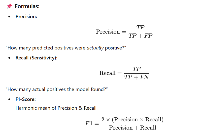
22️⃣ Precision, Recall, and F1-Score
Derived directly from the confusion matrix.
Python Code:
from sklearn.metrics import precision_score, recall_score, f1_score

precision = precision_score(y_true, y_pred)
recall = recall_score(y_true, y_pred)
f1 = f1_score(y_true, y_pred)

print(f"Precision: {precision}, Recall: {recall}, F1 Score: {f1}")
23️⃣ What is the ROC Curve?
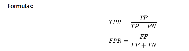
The ROC (Receiver Operating Characteristic) curve plots:
- TPR (Recall) vs
- FPR at different thresholds.
Interpretation:
- Curve close to top-left → excellent model
- Diagonal line → random guessing
Python Code:
from sklearn.metrics import roc_curve
import matplotlib.pyplot as plt

fpr, tpr, thresholds = roc_curve(y_true, y_scores)
plt.plot(fpr, tpr, label='ROC Curve')
plt.plot([0, 1], [0, 1], 'k--')
plt.xlabel('False Positive Rate')
plt.ylabel('True Positive Rate')
plt.title('ROC Curve')
plt.legend()
plt.show()
24️⃣ What is AUC-ROC?
AUC = Area Under the ROC Curve
Meaning:
- 1.0 → Perfect classifier
- 0.5 → Random guess
- > 0.5 → Useful model
AUC measures the overall ability to distinguish between classes.
Code:
from sklearn.metrics import roc_auc_score

auc = roc_auc_score(y_true, y_scores)
print(f"AUC-ROC Score: {auc}")
25️⃣ Choosing the Right Evaluation Metric
Depends on your domain + cost of mistakes.
📌 Recommended Metrics Based on Problem:
| Scenario | Best Metric |
|---|---|
| Balanced data | Accuracy |
| Imbalanced data | Precision, Recall, F1, AUC |
| Medical diagnosis (avoid FN) | Recall |
| Spam detection (avoid FP) | Precision |
| Multi-class | Macro/Micro F1, Accuracy |
| Need probability quality | Log Loss, AUC |
Example:
🔹 Medical tests: Missing a disease = worst → choose Recall
🔹 Spam filtering: Marking important email as spam = worst → choose Precision
26️⃣ Difference Between L1 & L2 Regularization
| Feature | L1 (Lasso) | L2 (Ridge) |
|---|---|---|
| Penalty | ( \lambda \sum | w_i |
| Sparsity | Produces sparse models (sets weights → 0) | Shrinks weights, does not zero them |
| Use Case | Feature selection | Prevent overfitting |
| Optimization | Not differentiable at 0 | Smooth & differentiable |
| Effect | Removes irrelevant features | Stabilizes weights |
Python Code
from sklearn.linear_model import Lasso, Ridge

# L1 Regularization (Lasso)
lasso = Lasso(alpha=0.1)
lasso.fit(X_train, y_train)

# L2 Regularization (Ridge)
ridge = Ridge(alpha=0.1)
ridge.fit(X_train, y_train)
27️⃣ How to Handle Imbalanced Datasets
When one class dominates heavily (e.g., fraud detection).
Techniques:
✅ 1. Resampling
- Oversampling → SMOTE
- Undersampling → remove majority samples
from imblearn.over_sampling import SMOTE
smote = SMOTE()
X_res, y_res = smote.fit_resample(X, y)
✅ 2. Use Correct Metrics
- F1-score
- Precision/Recall
- AUC-ROC
✅ 3. Class Weighting
from sklearn.linear_model import LogisticRegression
model = LogisticRegression(class_weight='balanced')
✅ 4. Ensemble Models
- Random Forest
- XGBoost (
scale_pos_weight)
✅ 5. Anomaly Detection
For extremely rare positive classes.
28️⃣ Purpose of a Learning Curve
A learning curve shows model performance as training data increases.
📌 Helps identify:
- Underfitting (both curves low)
- Overfitting (large gap between curves)
- Whether adding more data helps
Python Code
from sklearn.model_selection import learning_curve
import numpy as np
import matplotlib.pyplot as plt

train_sizes, train_scores, test_scores = learning_curve(
    estimator=model,
    X=X, y=y,
    train_sizes=np.linspace(0.1, 1.0, 10),
    cv=5,
    scoring="accuracy"
)

train_mean = train_scores.mean(axis=1)
test_mean = test_scores.mean(axis=1)

plt.plot(train_sizes, train_mean, label='Training score')
plt.plot(train_sizes, test_mean, label='Validation score')
plt.xlabel('Training Set Size')
plt.ylabel('Accuracy')
plt.title('Learning Curve')
plt.legend()
plt.show()
29️⃣ Detecting & Fixing Multicollinearity
Multicollinearity = independent variables are highly correlated, causing unstable coefficients.
How to detect:
🔹 1. Correlation Matrix
Look for > 0.8 correlations.
🔹 2. VIF — Variance Inflation Factor
- VIF > 10 = Serious multicollinearity
- VIF > 5 = Warning
VIF Code
from statsmodels.stats.outliers_influence import variance_inflation_factor
import pandas as pd

def compute_vif(df):
    vif_data = pd.DataFrame()
    vif_data["Feature"] = df.columns
    vif_data["VIF"] = [variance_inflation_factor(df.values, i)
                       for i in range(df.shape[1])]
    return vif_data

vif_df = compute_vif(X)
print(vif_df)
Fixes:
- Remove correlated features
- Use PCA
- Use regularization (L1/L2)
- Combine features
30️⃣ Difference Between Bagging & Boosting
| Feature | Bagging | Boosting |
|---|---|---|
| Type | Parallel ensemble | Sequential ensemble |
| Goal | Reduce variance | Reduce bias |
| Training | Independent models | Each model fixes previous errors |
| Best For | High-variance models | Weak models needing improvement |
| Robustness | Good with noisy data | Sensitive to outliers |
| Examples | Random Forest | AdaBoost, XGBoost, Gradient Boosting |
Bagging Example (Random Forest)
from sklearn.ensemble import RandomForestClassifier

rf = RandomForestClassifier(n_estimators=100)
rf.fit(X_train, y_train)
Boosting Example (AdaBoost)
from sklearn.ensemble import AdaBoostClassifier

ada = AdaBoostClassifier(n_estimators=100)
ada.fit(X_train, y_train)
31. What is feature engineering, and why is it important?
Definition:
Feature engineering is the process of creating, transforming, or selecting features from raw data to improve the performance of machine learning models.
Why It’s Important:
- ✔ Improves model accuracy and generalization
- ✔ Helps algorithms learn patterns more effectively
- ✔ Reduces overfitting by removing unnecessary features
- ✔ Speeds up training time and convergence
- ✔ Makes the model more interpretable
Common Feature Engineering Techniques:
- Creating new features (ratios, interactions, polynomial features)
- Transformations (log, square root, scaling)
- Binning continuous variables
- Encoding categorical features
- Handling missing values
- Feature selection (filter, wrapper, embedded methods)
32. How do you handle categorical variables in a dataset?
Categorical variables must be converted to numeric form before model training.
Encoding Techniques:
| Method | Description | Best For |
|---|---|---|
| Label Encoding | Assigns an integer to each category | Ordinal data (Low < Medium < High) |
| One-Hot Encoding | Creates binary column for each category | Nominal data (no order) |
| Target Encoding | Replaces category with target mean | High-cardinality features (hundreds of categories) |
Code Example:
from sklearn.preprocessing import LabelEncoder

le = LabelEncoder()
df['category_encoded'] = le.fit_transform(df['category'])
33. What is one-hot encoding?
One-hot encoding converts a categorical variable into multiple binary indicator variables.
Example:
| Color | red | green | blue |
|---|---|---|---|
| red | 1 | 0 | 0 |
| green | 0 | 1 | 0 |
| blue | 0 | 0 | 1 |
Code Examples:
Using Pandas
df_encoded = pd.get_dummies(df, columns=['color'])
Using Scikit-learn
from sklearn.preprocessing import OneHotEncoder
encoder = OneHotEncoder()
encoded_features = encoder.fit_transform(df[['color']])
34. Explain the concept of feature scaling and normalization.
Feature scaling transforms numerical values into a standard range so that each feature contributes equally.
Why It Is Needed
- Prevents dominance of large-range features
- Essential for distance-based algorithms:
✔ k-NN, ✔ SVM, ✔ K-Means - Required for gradient descent (Neural networks)
Common Techniques:
- Min-Max Scaling (Normalization) → range [0, 1]
- Standardization (Z-score Scaling) → mean 0, variance 1
35. Difference between Normalization and Standardization
| Feature | Normalization (Min-Max) | Standardization (Z-score) |
|---|---|---|
| Formula | (x − min) / (max − min) | (x − μ) / σ |
| Range | [0, 1] | No fixed range |
| Sensitive to outliers | Yes | Less sensitive |
| When to use | When data is not normal | When data follows Gaussian distribution |
Code Example:
from sklearn.preprocessing import MinMaxScaler, StandardScaler

# Normalization
minmax_scaler = MinMaxScaler()
X_norm = minmax_scaler.fit_transform(X)

# Standardization
std_scaler = StandardScaler()
X_std = std_scaler.fit_transform(X)
36. How do you deal with outliers in your data?
Outliers can negatively affect model accuracy, especially in linear models and distance-based algorithms.
Detection Methods
- Boxplot & IQR Rule
- Outlier if:
- x < Q1 – 1.5 × IQR
- x > Q3 + 1.5 × IQR
- Outlier if:
- Z-score Method
- Values with |Z| > 3 considered outliers
- Visualization
- Scatter plots
- Histograms
- Boxplots
Treatment Options
- Remove outliers
- Cap/Floor extreme values (Winsorization)
- Apply transformations (log, sqrt)
- Use RobustScaler to reduce outlier impact
- Replace outliers with median/percentile values
Code Example
from scipy.stats import zscore
import numpy as np

# Z-score method
df_cleaned = df[(np.abs(zscore(df)) < 3).all(axis=1)]

# IQR method
Q1 = df.quantile(0.25)
Q3 = df.quantile(0.75)
IQR = Q3 - Q1
df_cleaned = df[~((df < (Q1 - 1.5*IQR)) | (df > (Q3 + 1.5*IQR))).any(axis=1)]
37. What is feature selection, and how is it performed?
Definition
Feature selection is the process of selecting the most relevant features to improve model performance and reduce dimensionality.
Why It’s Important
- Faster training
- Reduces overfitting
- Improves accuracy
- Increases interpretability
Feature Selection Approaches
| Method | Description | Examples |
|---|---|---|
| Filter Methods | Select features based on statistical tests | Correlation, Chi-square |
| Wrapper Methods | Test subsets using a model | RFE, Forward/Backward selection |
| Embedded Methods | Done inside the model training process | Lasso (L1), Decision Trees |
38. Describe the Recursive Feature Elimination (RFE) method.
RFE is a wrapper feature selection technique that removes features recursively based on model importance.
Steps
- Train a model
- Rank features by importance
- Remove the least important feature(s)
- Repeat until the desired number of features is reached
Code Example
from sklearn.feature_selection import RFE
from sklearn.ensemble import RandomForestClassifier

model = RandomForestClassifier()
rfe = RFE(estimator=model, n_features_to_select=5)
X_selected = rfe.fit_transform(X, y)
39. How does regularization help in feature selection?
Regularization adds a penalty to large coefficients and helps reduce overfitting.
L1 Regularization (Lasso)
- Encourages sparsity
- Sets some coefficients exactly zero
- Automatically performs feature selection
L2 Regularization (Ridge)
- Shrinks coefficients
- Does not eliminate them
- Helps reduce variance but not used for feature selection
Code Example
from sklearn.linear_model import Lasso

lasso = Lasso(alpha=0.1)
lasso.fit(X_train, y_train)

# Selected features (non-zero coefficients)
selected_features = X.columns[lasso.coef_ != 0]
40. What is the role of domain knowledge in feature engineering?
Domain knowledge helps create meaningful and relevant features.
Importance of Domain Knowledge
- Determines useful transformations
- Avoids irrelevant or misleading features
- Helps design interaction or derived features
- Improves model interpretability
Examples
- Healthcare: BMI bins, age groups, risk scores
- Finance: Volatility, rolling averages, stock returns
- NLP: TF-IDF, sentiment analysis, keyword density
- Time Series: Lag features, moving averages, day-of-week
41. What is hyperparameter tuning?
Hyperparameters are parameters set before training (example: learning rate, number of trees, max depth) and not learned from data.
Hyperparameter Tuning
The process of finding the best hyperparameter combination to maximize model performance.
Why It’s Important
- Greatly improves accuracy
- Prevents underfitting & overfitting
- Optimizes training time and model complexity
42. Describe the grid search method for hyperparameter tuning.
Grid Search performs an exhaustive search through all possible hyperparameter combinations.
How It Works
- Define a grid of parameters
- Train the model for every combination
- Use cross-validation to evaluate each
- Select the best parameters
Code Example
from sklearn.model_selection import GridSearchCV
from sklearn.ensemble import RandomForestClassifier

param_grid = {
    'n_estimators': [50, 100],
    'max_depth': [None, 10, 20],
    'min_samples_split': [2, 5]
}

grid_search = GridSearchCV(
    RandomForestClassifier(),
    param_grid,
    cv=5,
    scoring='accuracy'
)

grid_search.fit(X_train, y_train)

print("Best Parameters:", grid_search.best_params_)
print("Best Score:", grid_search.best_score_)
43. What is random search, and how does it differ from grid search?
Random Search selects random combinations of hyperparameters instead of testing all.
Key Differences
| Feature | Grid Search | Random Search |
|---|---|---|
| Search Type | Exhaustive | Random sampling |
| Speed | Slow for large grids | Faster, scalable |
| Coverage | Tests all combinations | May skip some |
| Useful When | Small grid | Large search space |
Code Example
from sklearn.model_selection import RandomizedSearchCV
from scipy.stats import randint, uniform
from sklearn.ensemble import RandomForestClassifier

param_dist = {
    'n_estimators': randint(50, 200),
    'max_depth': [None, 10, 20, 30],
    'min_samples_split': uniform(0.1, 0.9)
}

random_search = RandomizedSearchCV(
    RandomForestClassifier(),
    param_dist,
    n_iter=30,
    cv=5,
    scoring='accuracy'
)

random_search.fit(X_train, y_train)

print("Best Parameters:", random_search.best_params_)
44. Explain the concept of early stopping in model training.
Early stopping is a regularization technique that stops training when the validation loss stops improving.
How It Works
- Evaluate validation loss each epoch
- If no improvement for N epochs (patience), stop
- Restore the best weights
Benefits
- Prevents overfitting
- Reduces training time
- Produces a more generalizable model
Code Example (Keras)
from tensorflow.keras.callbacks import EarlyStopping

early_stop = EarlyStopping(
    monitor='val_loss',
    patience=5,
    restore_best_weights=True
)

history = model.fit(
    X_train,
    y_train,
    epochs=100,
    validation_split=0.2,
    callbacks=[early_stop]
)
45. How do you prevent overfitting in a model?
Overfitting happens when the model memorizes training data patterns—including noise—leading to poor generalization.
Techniques to Prevent Overfitting
| Method | Description |
|---|---|
| Regularization (L1/L2) | Limits large weights |
| Cross-validation | Ensures generalization |
| Pruning | Simplifies decision trees |
| Dropout | Randomly removes neurons in neural nets |
| Data Augmentation | Creates more training samples |
| Reduce Model Complexity | Use simpler models |
| Early Stopping | Stop training when no improvement |
46. What is dropout in neural networks?
Dropout is a regularization technique used in deep learning to reduce overfitting.
How It Works
- During training, randomly drops (deactivates) a fraction of neurons.
- Prevents the network from relying too much on specific neurons.
- Forces the model to learn redundant, generalized representations.
- During inference, all neurons are used but their outputs are scaled to maintain balance.
Code Example (Keras)
from tensorflow.keras.layers import Dense, Dropout
from tensorflow.keras.models import Sequential

model = Sequential([
    Dense(128, activation='relu'),
    Dropout(0.5),  # 50% dropout
    Dense(64, activation='relu'),
    Dropout(0.5),
    Dense(1, activation='sigmoid')
])
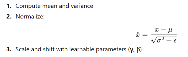
47. How does batch normalization work?
Batch Normalization (BatchNorm) normalizes the inputs of each layer to stabilize and speed up training.
Why It Helps
- Faster training & better convergence
- Reduces dependency on weight initialization
- Acts as a regularizer and reduces overfitting
How It Works (per mini-batch)
Code Example (Keras)
from tensorflow.keras.layers import Dense, BatchNormalization, Activation
from tensorflow.keras.models import Sequential

model = Sequential([
    Dense(128),
    BatchNormalization(),
    Activation('relu'),
    Dense(64),
    BatchNormalization(),
    Activation('relu'),
    Dense(1, activation='sigmoid')
])
48. What is the purpose of the activation function in neural networks?
Activation functions introduce non-linearity, allowing neural networks to learn complex patterns.
Why They Are Necessary
- Without activation functions, a neural network behaves like a linear model, no matter how many layers it has.
- Non-linearity helps the model learn curved boundaries, interactions, and complex features.
Common activation functions: ReLU, sigmoid, tanh, softmax, etc.
49. Compare and contrast different activation functions (ReLU, sigmoid, tanh).
Comparison Table
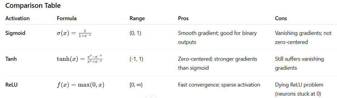
Optional Visualization Code
import matplotlib.pyplot as plt
import numpy as np

x = np.linspace(-5, 5, 100)

plt.plot(x, 1/(1 + np.exp(-x)), label="Sigmoid")
plt.plot(x, np.tanh(x), label="Tanh")
plt.plot(x, np.maximum(0, x), label="ReLU")

plt.legend()
plt.title("Activation Functions")
plt.grid(True)
plt.show()
50. What is the vanishing gradient problem, and how is it addressed?
The vanishing gradient problem occurs when gradients become extremely small during backpropagation, slowing or stopping learning—common in deep networks.
Causes
- Sigmoid/tanh saturate at large values → tiny gradients
- Very deep architectures
- Poor weight initialization
Solutions
- Use ReLU or variants (Leaky ReLU, ELU)
- Apply Batch Normalization
- Use skip connections (ResNet)
- Use He or Xavier initialization
- Avoid excessively deep networks
Example Fix
# Instead of:
Dense(64, activation='sigmoid')

# Use:
Dense(64, activation='relu')
51️⃣ Difference Between Shallow vs Deep Neural Networks
| Feature | Shallow NN | Deep NN |
|---|---|---|
| Hidden Layers | 1–2 | Many (10 to 100+) |
| Learning Ability | Simple patterns | Hierarchical complex features |
| Use Cases | Small datasets (Iris) | Images, NLP, voice |
| Training Time | Fast | Slow + compute heavy |
| Examples | Simple MLP | CNNs, RNNs, Transformers |
Example:
- Shallow NN: Can solve simple classification tasks.
- Deep NN: ImageNet-level CNNs, GPT/Transformers.
52️⃣ Architecture of a CNN (Convolutional Neural Network)
A CNN processes image-like grid data using filters.
Standard CNN Flow
- Input Layer → e.g., image (64×64×3)
- Conv Layer → feature extraction
- ReLU → non-linearity
- MaxPooling → reduces size
- Conv + Pool (repeat)
- Flatten → convert to vector
- Dense Layers → classification
Code Example (Keras)
from tensorflow.keras.models import Sequential
from tensorflow.keras.layers import Conv2D, MaxPooling2D, Flatten, Dense

model = Sequential([
    Conv2D(32, (3, 3), activation='relu', input_shape=(64, 64, 3)),
    MaxPooling2D((2, 2)),
    Conv2D(64, (3, 3), activation='relu'),
    MaxPooling2D((2, 2)),
    Flatten(),
    Dense(64, activation='relu'),
    Dense(10, activation='softmax')
])

model.summary()
Output (Model Summary — simplified):
Layer (type)        Output Shape      Param #
------------------------------------------------
Conv2D              (None, 62,62,32)   896
MaxPooling2D        (None, 31,31,32)   0
Conv2D              (None, 29,29,64)   18496
MaxPooling2D        (None, 14,14,64)   0
Flatten             (None, 12544)      0
Dense               (None, 64)         803,840
Dense               (None, 10)         650
------------------------------------------------
Total params: ~824K
53️⃣ How RNNs Handle Sequential Data
RNNs are designed for time-dependent data such as text, speech, and time series.
Key Ideas
- Maintain hidden state across time.
- At each step:
hₜ = f(xₜ, hₜ₋₁) - Can capture short-term dependencies.
Limitations
- Vanishing gradients → poor long-term memory.
Better Variants
- LSTM → long-term memory via gates
- GRU → simpler but effective gate design
Code Example (LSTM)
from tensorflow.keras.models import Sequential
from tensorflow.keras.layers import Embedding, LSTM, Dense

model = Sequential([
    Embedding(input_dim=10000, output_dim=64),
    LSTM(128),
    Dense(1, activation='sigmoid')
])

model.compile(optimizer='adam', loss='binary_crossentropy', metrics=['accuracy'])
Output (Model Summary — simplified):
Layer (type)      Output Shape       Param #
------------------------------------------------
Embedding         (None, None, 64)     640,000
LSTM              (None, 128)          98,816
Dense             (None, 1)            129
------------------------------------------------
Total params: ~739K
54️⃣ Role of the Embedding Layer in NLP
✔ Converts word IDs → dense vector representations
✔ Captures semantic meaning
✔ Reduces dimensionality vs one-hot encoding
✔ Enables relationships like:
king – man + woman ≈ queen
Popular Embeddings
- Word2Vec
- GloVe
- fastText
- BERT (contextual embeddings)
Code Example
from tensorflow.keras.layers import Embedding

embedding_layer = Embedding(
    input_dim=10000,
    output_dim=64,
    input_length=100
)
Output Shapes
- Input:
(batch_size, 100) - Output:
(batch_size, 100, 64)
55️⃣ What is Transfer Learning?
Transfer Learning = Using a pre-trained model (trained on a huge dataset like ImageNet) and fine-tuning it for your own task.
How it Works
- Load a pre-trained model
- Freeze early layers (generic features like edges, textures)
- Train top layers on your dataset (specific patterns)
Benefits
✔ Saves training time
✔ Works well even with small datasets
✔ Better generalization
56️⃣ What Are Pre-trained Models & How Are They Used?
Pre-trained models = Models already trained on large datasets (ImageNet, Wikipedia, COCO) that you can reuse.
Popular Pre-trained Models
Vision: VGG16, ResNet, EfficientNet, Inception
NLP: BERT, GPT, RoBERTa, DistilBERT
Use Cases
- ✔ Feature extraction
- ✔ Fine-tuning
- ✔ Transfer learning
Code Example — Using VGG16
from tensorflow.keras.applications import VGG16
from tensorflow.keras.models import Model
from tensorflow.keras.layers import GlobalAveragePooling2D, Dense

base_model = VGG16(weights='imagenet', include_top=False, input_shape=(224,224,3))

# Freeze base model
for layer in base_model.layers:
    layer.trainable = False

# Custom head
x = GlobalAveragePooling2D()(base_model.output)
x = Dense(1024, activation='relu')(x)
output = Dense(num_classes, activation='softmax')(x)

model = Model(inputs=base_model.input, outputs=output)
57️⃣ What is Backpropagation?
Backpropagation is the algorithm used to train neural networks by updating weights based on errors.
Steps
- Forward Pass: Compute predictions
- Loss Calculation: Compare with true label
- Backward Pass: Compute gradients (using chain rule)
- Weight Update: Apply gradient descent
Conceptually
- Compute ∂L/∂w (sensitivity of loss to weight change)
- Update:
w ← w − η × gradient
Where:
- L = Loss
- η = Learning rate
- w = weights
58️⃣ SGD vs Batch Gradient Descent
| Feature | Batch GD | Stochastic GD (SGD) |
|---|---|---|
| Data per update | Entire dataset | One sample |
| Speed | Slow | Fast |
| Stability | Stable, smooth | Noisy updates |
| Convergence | Exact minimum | Approximate |
| Memory | High | Low |
Mini-Batch GD
➡ Uses small batches (e.g., 32, 64)
➡ Best of both worlds: faster + stable
59️⃣ How to Choose the Right Optimizer?
| Optimizer | Description | Best For |
|---|---|---|
| SGD | Basic; stable | Small data, simple models |
| Adam | Adaptive LR + momentum | Most deep learning tasks |
| RMSProp | Good for non-stationary tasks | RNNs, time series |
| Adagrad | Large updates for rare features | NLP, embeddings |
| Adadelta | Fixes Adagrad’s decreasing LR | NLP |
Code Example
from tensorflow.keras.optimizers import Adam, SGD

# Adam
optimizer = Adam(learning_rate=0.001)

# SGD + momentum
optimizer = SGD(learning_rate=0.01, momentum=0.9)

model.compile(optimizer=optimizer, loss='categorical_crossentropy')
60️⃣ Challenges in Training Deep Neural Networks
| Challenge | Description | Solution |
|---|---|---|
| Vanishing/Exploding Gradients | Gradients shrink or blow up | ReLU, BatchNorm, Residual Blocks |
| Overfitting | Model memorizes data | Dropout, Early stopping, Regularization |
| Computational Cost | Too many params | GPUs, TPUs, distributed training |
| Data Scarcity | Deep nets need big datasets | Transfer learning, Data augmentation |
| Hyperparameter Tuning | Hard to find optimal settings | Grid search, Bayesian optimization |
61️⃣ Difference Between Clustering & Classification
| Feature | Clustering (Unsupervised) | Classification (Supervised) |
|---|---|---|
| Input | Only features (X) | Features + labels (X + y) |
| Goal | Discover hidden patterns/groups | Predict known class labels |
| Output | Cluster IDs | Class predictions |
| Examples | Customer segmentation | Spam detection |
Examples
- Clustering: Segment customers by purchase behavior
- Classification: Predict whether an email is spam / not spam
62️⃣ Describe DBSCAN Algorithm
DBSCAN = Density-Based Spatial Clustering of Applications with Noise
Best for arbitrarily-shaped clusters & outliers detection.
Key Parameters
- ε (epsilon): Neighborhood radius
- MinPts: Minimum points to form a dense region
How It Works
- A point is a core point if ≥ MinPts fall inside radius ε
- Core points → connected into clusters
- Non-reachable points → noise / outliers
Advantages
✔ Detects noise
✔ Works on arbitrary shapes
✔ No need to specify number of clusters
Code Example
from sklearn.cluster import DBSCAN
from sklearn.datasets import make_blobs

X, y = make_blobs(n_samples=300, centers=4, random_state=42)

dbscan = DBSCAN(eps=0.5, min_samples=5)
labels = dbscan.fit_predict(X)
63️⃣ How to Determine Optimal Number of Clusters in K-Means?
Methods
1. Elbow Method
- Plot inertia vs k
- Choose point where curve “bends”
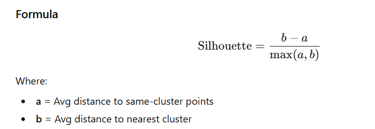
2. Silhouette Score
- Measures similarity within cluster vs nearest cluster
- Higher = better
Elbow Method Code
from sklearn.cluster import KMeans
import matplotlib.pyplot as plt

inertias = []
for k in range(1, 11):
    kmeans = KMeans(n_clusters=k, random_state=42)
    kmeans.fit(X)
    inertias.append(kmeans.inertia_)

plt.plot(range(1, 11), inertias, marker='o')
plt.xlabel('Number of clusters')
plt.ylabel('Inertia')
plt.title('Elbow Method')
plt.show()
64️⃣ What is Silhouette Score?
Silhouette Score tells how well each point fits in its cluster.
Interpretation
| Score | Meaning |
|---|---|
| +1 | Perfectly clustered |
| 0 | On the cluster boundary |
| −1 | Misclassified |
Code Example
from sklearn.metrics import silhouette_score

kmeans = KMeans(n_clusters=4)
labels = kmeans.fit_predict(X)

score = silhouette_score(X, labels)
print("Silhouette Score:", score)
65️⃣ Explain Anomaly Detection
Anomaly detection identifies rare, unusual, or suspicious data points.
Use Cases
- Fraud detection
- Credit card scams
- Cybersecurity
- Manufacturing defects
Types
| Method | Description |
|---|---|
| Supervised | Labeled normal + anomaly data |
| Semi-supervised | Train only on normal data |
| Unsupervised | No labels; detect points far from density |
Approaches
- Distance-based (KNN)
- Density-based (DBSCAN, LOF)
- Reconstruction error (Autoencoders)
- Statistical (Z-score, Gaussian models)
✅ 66. How does the Isolation Forest algorithm work?
Isolation Forest is an anomaly detection method based on the idea that anomalies are easier to isolate than normal points.
Key Intuition
- Anomalies = few & different → require fewer splits to isolate
- Build many random isolation trees
- Short average path length → anomaly
- Long path length → normal point
Code Example
from sklearn.ensemble import IsolationForest

iso_forest = IsolationForest(contamination=0.1)  # Fraction of anomalies
iso_forest.fit(X)

anomalies = iso_forest.predict(X)  # -1 = anomaly, 1 = normal
✅ 67. What are Gaussian Mixture Models (GMMs)?
A Gaussian Mixture Model (GMM) assumes that the data is generated from a mixture of multiple Gaussian (normal) distributions.
Key Points
- Each cluster = one Gaussian distribution
- Performs soft clustering → each point gets a probability for each cluster
- Uses Expectation-Maximization (EM) to find means, variances, and mixing weights
Code Example
from sklearn.mixture import GaussianMixture

gmm = GaussianMixture(n_components=4, random_state=42)
gmm.fit(X)

probs = gmm.predict_proba(X)  # Soft probabilities
✅ 68. Compare K-Means and GMMs
| Feature | K-Means | GMM |
|---|---|---|
| Type | Hard clustering | Soft clustering |
| Cluster Shape | Spherical | Elliptical (more flexible) |
| Distribution Assumption | None | Gaussian distribution |
| Output | Single cluster label | Probability of belonging to each cluster |
| Sensitivity | Sensitive to centroid init | More robust |
| Complexity | Simple | More complex (covariance matrices) |
Summary:
K-Means is simple & fast; GMM is more flexible & probabilistic.
✅ 69. What is the Expectation–Maximization (EM) algorithm?
EM is an iterative optimization algorithm used for models with latent (hidden) variables.
Two-Step Cycle
- E-step:
Estimate expected log-likelihood using current parameters. - M-step:
Maximize this expected log-likelihood to update parameters.
Repeat until convergence.
Used in
- Gaussian Mixture Models
- Hidden Markov Models
- Missing data imputation
- Latent variable models
✅ 70. How do you evaluate the performance of clustering algorithms?
Clustering = unsupervised, so evaluation is tricky.
A) Internal Evaluation Metrics
(Do NOT require true labels)
1. Silhouette Score
Higher = better separation
2. Calinski–Harabasz Index
Higher = dense & well-separated clusters
3. Davies–Bouldin Index
Lower = better clusters
B) External Evaluation Metrics
(Require ground truth labels)
1. Adjusted Rand Index (ARI)
Measures similarity between cluster assignments and true labels
Range: [-1, 1]
2. Normalized Mutual Information (NMI)
Measures information shared between predicted and true labels
Range: [0, 1]
Code Example
from sklearn.metrics import adjusted_rand_score, normalized_mutual_info_score

true_labels = [0, 0, 1, 1, 2, 2]
predicted_labels = [1, 1, 0, 0, 2, 2]

ari = adjusted_rand_score(true_labels, predicted_labels)
nmi = normalized_mutual_info_score(true_labels, predicted_labels)

print("Adjusted Rand Index:", ari)
print("Normalized Mutual Info Score:", nmi)
✅ 71. What is a time series, and how is it different from other data types?
Time series: A sequence of data points recorded in chronological order.
Key Characteristics
- Temporal ordering: Order of data points matters.
- Autocorrelation: Current values often depend on past values.
- Trend & Seasonality: Patterns over time (long-term trends, repeating cycles).
Comparison with other data types
| Feature | Time Series | Cross-Sectional | Panel Data |
|---|---|---|---|
| Time Dependency | Yes | No | Partial (multiple entities over time) |
| Example | Stock prices over time | Customer age/gender | Sales across stores over time |
✅ 72. Describe the components of a time series
Most time series can be decomposed into four main components:
- Trend (T): Long-term upward or downward movement.
- Seasonality (S): Repeating short-term cycles (daily, weekly, monthly).
- Cyclical (C): Long-term fluctuations not of fixed period (e.g., business cycles).
- Irregular / Noise (I): Random variation unexplained by other components.
Code Example
from statsmodels.tsa.seasonal import seasonal_decompose
import matplotlib.pyplot as plt

result = seasonal_decompose(data, model='multiplicative', period=12)
result.plot()
plt.show()
✅ 73. What is stationarity in time series data?
A time series is stationary if its statistical properties (mean, variance, autocorrelation) remain constant over time.
Why Stationarity Matters
- Most classical forecasting models (ARIMA, etc.) assume stationarity.
- Stationary series are easier to model and forecast accurately.
Types of Stationarity
- Strict Stationarity: Full distribution invariant to time shifts.
- Weak (Covariance) Stationarity: Mean, variance, and autocovariance are constant.
✅ 74. How do you test for stationarity?
1. Visual Inspection
- Plot rolling mean & rolling standard deviation.
- Look for trends or seasonality.
2. Statistical Tests
Augmented Dickey-Fuller (ADF) Test
- Null hypothesis H0H_0H0: Unit root exists → non-stationary
- Reject H0H_0H0 if p-value < 0.05 → stationary
Code Example
from statsmodels.tsa.stattools import adfuller

def adf_test(series):
    result = adfuller(series)
    print('ADF Statistic:', result[0])
    print('p-value:', result[1])
    print('Critical Values:')
    for key, value in result[4].items():
        print(f'   {key}: {value}')

adf_test(data)
✅ 75. Explain the Autoregressive Integrated Moving Average (ARIMA) model
ARIMA(p, d, q) is a widely used model for univariate time series forecasting.
Parameters
- p: Number of autoregressive terms (AR) – depends on past values.
- d: Degree of differencing to make series stationary (I).
- q: Number of moving average terms (MA) – depends on past forecast errors.
How It Works
- AR(p): Predicts using past values.
- I(d): Differencing removes trend/seasonality.
- MA(q): Predicts using past errors.
Code Example
from statsmodels.tsa.arima.model import ARIMA

model = ARIMA(train_data, order=(1,1,1))  # ARIMA(1,1,1)
results = model.fit()
forecast = results.forecast(steps=10)
✅ 76. Difference between AR, MA, and ARIMA models
| Model | Description | Use Case |
|---|---|---|
| AR(p) | Autoregressive model; predicts current value using past values. | When current values depend on their own history. |
| MA(q) | Moving Average model; predicts current value using past forecast errors. | When current value depends on errors of previous predictions. |
| ARIMA(p,d,q) | Combines AR + I (integration/differencing) + MA. | For non-stationary time series where differencing is needed. |
✅ 77. Handling seasonality in time series data
Approaches:
- Seasonal Decomposition: Remove seasonal component to analyze trend & residuals.
- Seasonal Differencing: Subtract value from previous season (e.g.,
y_t - y_{t-12}for monthly data). - Seasonal Models: Use models like SARIMA:
- SARIMA(p,d,q)(P,D,Q)m
m= number of periods per season (e.g., 12 for monthly data)
Code Example (SARIMA)
from statsmodels.tsa.statespace.sarimax import SARIMAX

# SARIMA(1,1,1)(1,1,1,12)
model = SARIMAX(data, order=(1,1,1), seasonal_order=(1,1,1,12))
results = model.fit()
forecast = results.get_forecast(steps=12)
✅ 78. Exponential Smoothing
Exponential smoothing assigns decreasing weights to older observations.
Types
- Simple Exponential Smoothing (SES): Captures level only.
- Holt’s Linear Trend Method: Level + trend.
- Holt-Winters Method: Level + trend + seasonality.
Code Example (Holt-Winters)
from statsmodels.tsa.holtwinters import ExponentialSmoothing

model = ExponentialSmoothing(data, trend='multiplicative',
                             seasonal='multiplicative', seasonal_periods=12)
fit = model.fit()
forecast = fit.forecast(steps=12)
✅ 79. Lag in time series analysis
- Lag: Shifting the time series by one or more periods.
- Lag-1: Uses value at t-1 to predict value at t.
- Uses:
- Autocorrelation analysis
- Feature engineering for models like LSTMs or AR models
Code Example (Create Lag Features)
data['lag1'] = data['value'].shift(1)
data['lag2'] = data['value'].shift(2)
print(data[['value', 'lag1', 'lag2']].head())
✅ 80. Evaluating accuracy of time series forecasts

Code Example
from sklearn.metrics import mean_absolute_error, mean_squared_error
import numpy as np
mae = mean_absolute_error(test, forecast)
mse = mean_squared_error(test, forecast)
rmse = mean_squared_error(test, forecast, squared=False)
mape = np.mean(np.abs((test - forecast) / test)) * 100
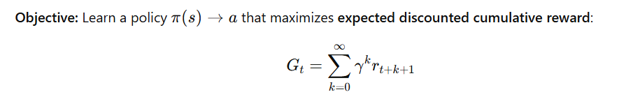
print(f"MAE: {mae}, MSE: {mse}, RMSE: {rmse}, MAPE: {mape:.2f}%")✅ 81. What is Reinforcement Learning (RL)?
Definition:
Reinforcement Learning is a type of machine learning where an agent learns by interacting with an environment, taking actions to maximize cumulative reward over time.
Key Components
| Component | Description |
|---|---|
| Agent | The learner or decision-maker that performs actions. |
| Environment | The world or system the agent interacts with. |
| State (s) | Representation of the current situation in the environment. |
| Action (a) | Choices the agent can make at each state. |
| Reward (r) | Feedback received after taking an action; guides learning. |
| Policy (π) | Strategy that maps states to actions. |
| Value Function (V(s)) | Expected cumulative reward from a given state. |
| Q-Function (Q(s,a)) | Expected cumulative reward from a state-action pair. |
How RL Works
- Agent observes the current state of the environment.
- Agent chooses an action based on its policy.
- Environment returns a reward and updates to a new state.
- Agent updates its policy/value function to improve future decisions.
- Repeat until the agent learns an optimal strategy.

Example Use Cases
- Games: AlphaGo, Chess, Atari games
- Robotics: Teaching robots to walk or pick objects
- Finance: Portfolio management, trading strategies
- Recommendation Systems: Personalized content selection
82. Exploration vs. Exploitation Dilemma
In RL, the agent must balance between:
| Strategy | Description |
|---|---|
| Exploration | Try new actions to discover potentially better rewards. |
| Exploitation | Use known actions that currently yield the highest reward. |
Why it matters:
- Pure exploitation may miss better rewards.
- Pure exploration wastes time on suboptimal actions.
Common Strategies to Balance:
- ε-greedy:
- With probability ε, choose a random action (explore).
- With probability 1-ε, choose the best-known action (exploit).
- Softmax (Boltzmann Exploration):
- Select actions probabilistically based on estimated Q-values.
- Upper Confidence Bound (UCB):
- Chooses actions with the highest upper bound of expected reward, balancing uncertainty.
83. Markov Decision Processes (MDPs)
Definition:
MDPs are a mathematical framework for modeling sequential decision-making where outcomes are partly random and partly under control.
Components:
| Component | Description |
|---|---|
| States (S) | All possible situations the agent can be in. |
| Actions (A) | Choices available to the agent. |
| **Transition Model P(s’ | s, a)** |
| Reward Function R(s, a, s’) | Immediate reward received after taking action a in state s and transitioning to s’. |
| Discount Factor γ | Weight for future rewards (0 ≤ γ ≤ 1). |
84. Q-Learning
Definition:
Q-learning is a model-free, off-policy RL algorithm that learns the optimal action-value function Q(s,a)Q(s, a)Q(s,a) without needing a model of the environment.
How it works:

Python Example (FrozenLake):
import gym
import numpy as np

env = gym.make('FrozenLake-v1')
q_table = np.zeros([env.observation_space.n, env.action_space.n])

alpha = 0.8   # learning rate
gamma = 0.95  # discount factor
episodes = 2000

for _ in range(episodes):
    state = env.reset()
    done = False
    while not done:
        action = np.argmax(q_table[state])
        next_state, reward, done, info = env.step(action)
        q_table[state, action] += alpha * (reward + gamma * np.max(q_table[next_state]) - q_table[state, action])
        state = next_state
Notes:
- Off-policy means Q-learning learns the optimal policy independently of the agent’s actions.
- Converges to the optimal Q-values over time.
85. Role of the Reward Function in Reinforcement Learning
The reward function defines the agent’s objective by assigning feedback for each action in a given state. It essentially tells the agent what is “good” or “bad.”
Key Points:
- Guides the agent’s behavior toward desired goals.
- Must be informative, but not too sparse.
- Poorly designed rewards can lead to unintended behaviors.
Examples:
- Game: +1 for winning, -1 for losing, 0 otherwise.
- Robotics: Reward smooth movement, penalize energy use.
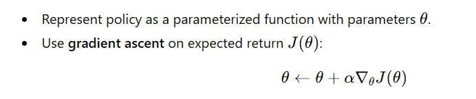
86. Policy Gradients
Policy gradient methods directly optimize the policy πθ(a∣s)\pi_\theta(a|s)πθ(a∣s) instead of estimating Q-values.
How it works:
Advantages:
- Works with continuous action spaces.
- Stochastic policies allow natural exploration.
Disadvantages:
- High variance in updates.
- Sample inefficient.
Popular Algorithms:
- REINFORCE
- Actor-Critic
- A2C (Advantage Actor-Critic)
87. Model-Based vs Model-Free RL
| Feature | Model-Based RL | Model-Free RL |
|---|---|---|
| Environment Model | Needs transition & reward model | Learns directly from experience |
| Planning | Can plan ahead using the model | No planning, learns policy/value directly |
| Efficiency | More sample-efficient | Less sample-efficient |
| Complexity | Harder to build accurate models | Simpler to implement |
| Examples | Dyna, PILCO | Q-learning, SARSA, DQN |
88. GAN Architecture
Generative Adversarial Networks consist of two networks competing:
- Generator (G): Creates fake data from random noise.
- Discriminator (D): Classifies real vs generated data.
Training Process:
- G tries to fool D by generating realistic samples.
- D tries to distinguish real from fake.
- Training continues until a Nash equilibrium is reached.
89. GANs vs Autoencoders
| Feature | GANs | Autoencoders |
|---|---|---|
| Goal | Generate realistic samples | Reconstruct input data |
| Architecture | Two competing networks | Encoder-decoder structure |
| Latent Space | Random noise (non-interpretable) | Encoded representation |
| Training | Adversarial (game-theoretic) | Minimize reconstruction loss |
| Output Quality | Often sharp and realistic | May be blurry |
| Stability | Hard to train, mode collapse issues | Generally stable |
90. Challenges in Training GANs
Common Challenges:
- Mode Collapse: Generator produces limited variety.
- Instability: Training oscillates or diverges.
- Vanishing Gradients: Discriminator becomes too strong.
- Evaluation Difficulty: No single metric for quality/diversity.
- Hyperparameter Sensitivity: Small changes can break training.
Solutions:
- Use Wasserstein GAN (WGAN) or WGAN-GP.
- Add gradient penalty.
- Alternate training of D and G.
- Apply spectral normalization.
- Monitor metrics like FID score.
91. How to Deploy a Machine Learning Model
Deploying a model moves it from development to production so it can make real-time predictions.
Key Steps:
- Model Training & Evaluation
- Train and validate the model locally using historical data.
- Ensure metrics meet business requirements.
- Model Serialization
- Save the trained model for reuse.
- Common formats:
pickle/joblib(Python)ONNX(cross-platform)
import joblib # Save trained model joblib.dump(model, 'model.pkl') # Load model in production loaded_model = joblib.load('model.pkl') - API Development
- Wrap the model in a REST or gRPC API.
- Use frameworks like Flask, FastAPI, or Django.
- Containerization
- Package the model and API in Docker for consistent environments.
- Cloud Hosting
- Deploy to platforms like AWS (SageMaker, EC2), GCP (AI Platform), Azure, or Heroku.
- Monitoring & Logging
- Track model performance, latency, and errors in real-time.
92. Common Challenges in Model Deployment
| Challenge | Description |
|---|---|
| Scalability | Efficiently handle high volumes of requests. |
| Latency | Ensure fast inference for real-time applications. |
| Versioning | Manage multiple versions of models and APIs. |
| Data Drift | Input data may change over time, reducing accuracy. |
| Security | Protect against adversarial attacks and unauthorized access. |
| Integration | Ensure compatibility with existing systems, databases, and pipelines. |
93. Monitoring Deployed Models
Monitoring ensures that models remain reliable and effective after deployment.
Key Metrics:
- Accuracy or other performance metrics over time.
- Prediction latency (speed of inference).
- Input data distribution shifts (detect data drift).
- Error rates or failed predictions.
- Confidence scores of predictions.
Tools:
- Prometheus + Grafana: Metrics collection and visualization.
- MLflow: Logging and model versioning.
- AWS CloudWatch: Monitoring on AWS.
- Azure Application Insights: Monitoring on Azure.
Example – Logging Predictions:
import logging
logging.basicConfig(filename='model_logs.log', level=logging.INFO)

def predict(input_data):
    prediction = model.predict(input_data)
    logging.info(f"Input: {input_data}, Prediction: {prediction}")
    return prediction
94. What is Model Drift, and How Do You Detect It?
Definition:
Model drift occurs when the statistical properties of input data or the relationship between input and output change over time, leading to degraded model performance.
Types of Drift:
- Concept Drift: Relationship between features and target changes.
- Example: Customer behavior changes over time.
- Data Drift: Input feature distribution changes.
- Example: Sensor readings gradually shift due to hardware aging.
Detection Methods:
- Statistical Tests:
- Kolmogorov-Smirnov (KS) Test, Chi-square test, etc.
- Monitoring Tools:
- Evidently AI, NannyML, WhyLogs.
- Performance Drop:
- Compare model performance metrics (accuracy, RMSE) over time against baseline.
Code Example (KS Test for Data Drift):
from scipy.stats import ks_2samp

# Compare train vs new data feature distributions
stat, p_value = ks_2samp(X_train['feature'], X_new['feature'])

if p_value < 0.05:
    print("Drift detected!")
else:
    print("No significant drift.")
95. How to Handle Real-Time Predictions
Real-time prediction systems must deliver low-latency responses for incoming requests.
Best Practices:
- Use lightweight or optimized models (LightGBM, small neural networks).
- Cache frequent responses to reduce computation.
- Use asynchronous processing for batch or queued inference.
- Optimize model inference using frameworks like ONNX, TensorRT, or TensorFlow Lite.
Code Example (FastAPI Real-Time Inference):
from fastapi import FastAPI
import joblib

app = FastAPI()
model = joblib.load("model.pkl")

@app.post("/predict")
def predict(data: dict):
    prediction = model.predict([data["features"]])
    return {"prediction": prediction.tolist()}
96. Role of APIs in Model Deployment
Definition:
APIs (Application Programming Interfaces) act as an interface for external applications to interact with your deployed model.
Benefits:
- Decouples model logic from application logic.
- Enables scalability and load balancing via RESTful or gRPC interfaces.
- Facilitates integration with mobile apps, web apps, dashboards, or other services.
Common Frameworks:
- Flask: Lightweight, simple to use.
- FastAPI: Fast, supports asynchronous requests.
- Tornado / Django REST Framework: Useful for high-performance or complex applications.
97. Ensuring Data Privacy and Security in ML Applications
Privacy Considerations:
- Data Anonymization: Remove personally identifiable information (PII) before training.
- Encryption: Use HTTPS/TLS for data in transit; encrypt stored data.
- Access Control: Role-based access, authentication, and audit logs.
- Compliance: Follow regulations like GDPR, HIPAA, CCPA.
Techniques:
- Federated Learning: Train models across decentralized data sources without sharing raw data.
- Differential Privacy: Add noise to data or gradients to prevent leakage of individual records.
- Secure Multi-party Computation: Joint computations without revealing private data.
Tools:
- IBM AI Fairness 360
- Google Differential Privacy Library
- TFX (TensorFlow Extended) for secure and reproducible pipelines
98. Ethical Considerations in Machine Learning
Key Issues:
- Bias & Discrimination: Models can reflect historical or dataset biases.
- Transparency: Black-box models can be hard to interpret.
- Accountability: Determining responsibility for harmful decisions.
- Surveillance & Consent: Avoid using personal data without consent.
- Environmental Impact: Large models consume significant compute and energy.
Frameworks & Initiatives:
- FAT Conference:* Fairness, Accountability, Transparency
- Partnership on AI
- Microsoft Fairlearn: Tools to assess fairness
99. Handling Bias in ML Models
Strategies:
- Audit Data: Check distributions across sensitive attributes (e.g., gender, race).
- Fairness Metrics: Use metrics like disparate impact or equal opportunity difference.
- Bias Mitigation Techniques:
- Reweighting: Adjust weights of samples during training.
- Adversarial Debiasing: Train models to minimize bias signal.
- Post-processing Calibration: Adjust predictions to improve fairness.
Code Example (Fairlearn):
from fairlearn.metrics import MetricFrame
from sklearn.metrics import accuracy_score

metric_frame = MetricFrame(
    metric=accuracy_score,
    y_true=y_test,
    y_pred=predictions,
    sensitive_features=sensitive_attr
)

print(metric_frame.overall)
print(metric_frame.by_group)
100. Best Practices for Maintaining and Updating Deployed Models
Key Practices:
- Continuous Monitoring: Track model performance and detect data drift.
- Retraining Pipelines: Automate retraining with new or fresh data.
- Version Control: Use DVC, MLflow, or Git to track model versions.
- Rollback Strategy: Keep older versions for fallback in case of failure.
- A/B Testing: Safely test new models in production with a subset of traffic.
- Documentation: Maintain logs, model metadata, and retraining history.
Code Example (Automated Retraining Trigger):
from datetime import datetime

last_retrain_date = datetime(2024, 1, 1)

if (datetime.now() - last_retrain_date).days > 30:
    print("Triggering retraining...")
    # Call retraining function here