What is a neural network, and what are its core components (e.g., layers, weights, biases)?

A neural network is a computational model inspired by the structure and function of the human brain. It’s composed of interconnected units called neurons , which work together to learn patterns from data. Neural networks are the foundational building blocks of deep learning

What Is a Neuron?

At the core of a neural network is the artificial neuron , which mimics how biological neurons process information.

Structure of a Neuron:

1. Inputs (x₁, x₂, …, xₙ) : Features or values coming into the neuron.
2. Weights (w₁, w₂, …, wₙ) : Parameters that determine the importance of each input.
3. Bias (b) : An additional parameter that shifts the output.
4. Weighted Sum : z=w1​x1+w2​x2​+⋯+wn​xn​+b
5. Activation Function (σ) : Applies non-linearity to the output. Common ones include:
   • Sigmoid
   • ReLU (Rectified Linear Unit)
   • Tanh

Final output of neuron:
y=σ(z)

📦 Core Components of a Neural Network

1. Layers

• Input Layer : Receives raw data (e.g., pixels of an image).
• Hidden Layers : Intermediate layers between input and output; extract features from data.
• Output Layer : Produces the final prediction.

The more hidden layers a network has, the “deeper” it is — hence the term deep learning .

2. Weights and Biases

• Weights : Control how strongly each input affects the neuron.
• Biases : Allow shifting the activation function left or right, improving flexibility.

These parameters are learned during training using optimization algorithms like Stochastic Gradient Descent (SGD) or Adam .

3. Activation Functions

Introduce non-linear properties to the network so it can learn complex patterns.

Common Activation Functions:

Name	Formula	Use Case
ReLU	max(0, x)	Most common in hidden layers
Sigmoid	1 / (1 + exp(-x))	Output layer for binary classification
Softmax	exp(x_i)/Σexp(x_j)	Output layer for multi-class classification

🔍 Example: A Simple Neural Network in Code

Let’s build a basic feedforward neural network with one hidden layer using TensorFlow/Keras.

import tensorflow as tf
from tensorflow.keras import layers, models

# Define a simple Sequential model
model = models.Sequential()

# Input layer + Hidden layer 1
model.add(layers.Dense(units=64, activation='relu', input_shape=(10,)))

# Output layer
model.add(layers.Dense(units=1, activation='sigmoid'))

# Compile the model
model.compile(optimizer='adam',
              loss='binary_crossentropy',
              metrics=['accuracy'])

# Summary of the model architecture
model.summary()

output:

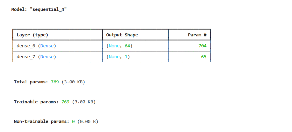
Explanation:

• Dense(64, activation='relu'): A fully connected layer with 64 neurons and ReLU activation.
• Dense(1, activation='sigmoid'): Output layer with 1 neuron and sigmoid activation (for binary classification).
• input_shape=(10,): Each input sample has 10 features.

Read : Machine Learning ?

📊 How Does Forward Propagation Work?

Let’s simulate forward propagation manually using NumPy:

import numpy as np

# Inputs (example: 3 features)
X = np.array([1.0, 2.0, 3.0])  # shape (3,)

# Weights (3 inputs -> 1 neuron)
W = np.array([0.5, -0.5, 0.2])  # shape (3,)
b = 0.1  # bias

# Compute weighted sum
z = np.dot(W, X) + b

# Apply activation function (ReLU)
a = np.maximum(0, z)

print("Weighted sum:", z)
print("Activated output:", a)

output:
Weighted sum: 0.2000000000000001
Activated output: 0.2000000000000001

This simulates what a single neuron does during forward propagation .

---

🎯 Training a Neural Network

The goal of training is to adjust weights and biases to minimize the loss function .

Key Steps:

1. Forward Pass : Make predictions.
2. Loss Calculation : Compare predictions to true labels.
3. Backpropagation : Calculate gradients of the loss with respect to weights.
4. Optimization : Update weights using gradient descent.

🧪 Real-World Applications

• Image Classification (CNNs)
• Speech Recognition (RNNs, Transformers)
• Time Series Forecasting (LSTMs)
• Game AI (Reinforcement Learning with Neural Networks)

---

✅ Summary

Component	Description
Neuron	Basic unit that computes weighted sum + activation
Layers	Group of neurons; includes input, hidden, and output layers
Weights & Biases	Learnable parameters adjusted during training
Activation Functions	Introduce non-linearity (ReLU, Sigmoid, etc.)
Training	Done via backpropagation and optimization algorithms

some other example

Example: A Simple Neural Network

Consider a neural network for predicting whether a house price is high (1) or low (0) based on two features: square footage and number of bedrooms.

• Input Layer: 2 nodes (square footage, bedrooms).
• Hidden Layer: 3 nodes (to learn intermediate patterns).
• Output Layer: 1 node (sigmoid activation for binary classification).
• Weights: Each connection (e.g., from input to hidden nodes) has a weight.
• Biases: Each hidden and output node has a bias.
• Activation: ReLU for hidden layers, sigmoid for the output layer.

The network learns to weigh features (e.g., larger square footage increases the likelihood of a high price) and adjust biases to fine-tune predictions.

Code Example: Building a Simple Neural Network

Let’s implement a neural network for binary classification using Python and TensorFlow/Keras. We’ll use a synthetic dataset to predict whether a point lies above or below a line (a simple binary classification task).

import numpy as np
import tensorflow as tf
from tensorflow.keras import layers, models
import matplotlib.pyplot as plt

# Generate synthetic data
np.random.seed(42)
X = np.random.rand(1000, 2)  # 1000 points with 2 features
y = (X[:, 0] + X[:, 1] > 1).astype(int)  # Class 1 if sum > 1, else 0

# Build neural network
model = models.Sequential([
    layers.Dense(4, activation='relu', input_shape=(2,)),  # Hidden layer with 4 neurons
    layers.Dense(1, activation='sigmoid')  # Output layer for binary classification
])

# Compile model
model.compile(optimizer='adam', loss='binary_crossentropy', metrics=['accuracy'])

# Train model
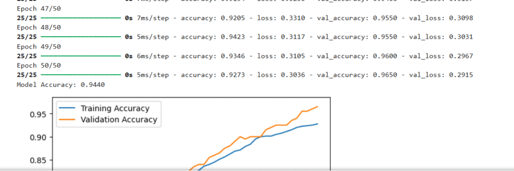
history = model.fit(X, y, epochs=50, batch_size=32, validation_split=0.2, verbose=1)

# Evaluate
loss, accuracy = model.evaluate(X, y, verbose=0)
print(f"Model Accuracy: {accuracy:.4f}")

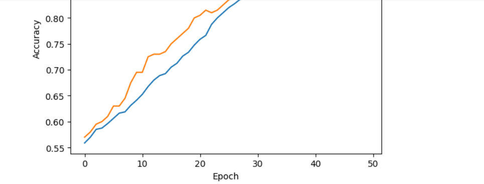
# Visualize training history
plt.plot(history.history['accuracy'], label='Training Accuracy')
plt.plot(history.history['val_accuracy'], label='Validation Accuracy')
plt.xlabel('Epoch')
plt.ylabel('Accuracy')
plt.legend()
plt.show()

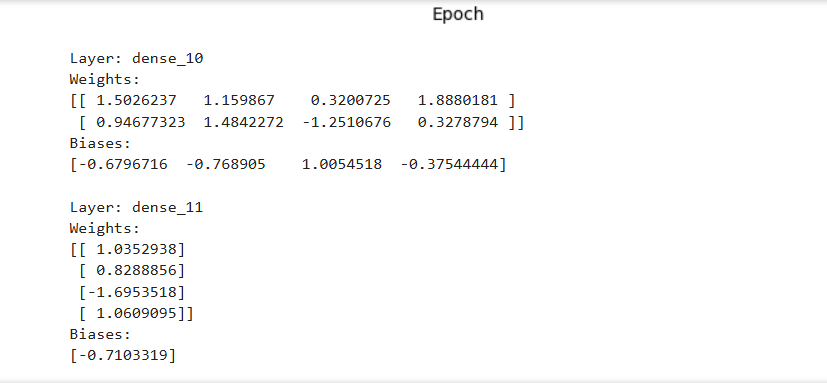
# Inspect weights and biases
for layer in model.layers:
    weights, biases = layer.get_weights()
    print(f"Layer: {layer.name}")
    print(f"Weights:\n{weights}")
    print(f"Biases:\n{biases}\n")

Explanation of Code:

• Data: 1000 points with 2 features (randomly generated). The label is 1 if the sum of features exceeds 1, else 0.
• Model:
  • Input layer: 2 features (implicit).
  • Hidden layer: 4 neurons with ReLU activation (weights: 2×4 matrix, biases: 4 values).
  • Output layer: 1 neuron with sigmoid activation (weights: 4×1 matrix, bias: 1 value).
• Training: Uses Adam optimizer and binary cross-entropy loss. Trains for 50 epochs.
• Output:
  • Prints model accuracy (e.g., ~0.95, indicating good performance).
  • Plots training and validation accuracy over epochs.
  • Displays weights and biases for each layer, showing how the network learned to separate classes.

Sample Output: